2Orientation for the Bio-CuriousThe Basics of Biology for the Physical Scientist
If you want to understand function, study structure. [I was supposed to have said in my molecular biology days.]
—Francis Crick, What Mad Pursuit: A Personal View of Scientific Discovery (1988, p. 150)
General Idea: This chapter outlines the essential details of the life sciences that physical scientists need to get to grips with, including the architecture of organisms, tissues, cells, and biomolecules as well as the core concepts of processes such as the central dogma of molecular biology, and discusses the key differences in the scientific terminology of physical parameters.
2.1 Introduction: The Material Stuff of Life
The material properties of living things for many physical scientists can be summarized as those of soft condensed matter. This phrase describes a range of physical states that in essence are relatively easily transformed or deformed by thermal energy fluctuations at or around room temperature. This means that the free energy scale of transitions between different physical states of the soft condensed matter is similar to those of the thermal reservoir of the system, namely, that of ∼kBT, where kB is the Boltzmann constant of 1.38 × 10⁻²³ m2 kg s−2 K−1 at absolute temperature T. In the case of this living soft condensed matter, the thermal reservoir can be treated as the surrounding water solvent environment. However, a key feature of living soft matter is that it is not in thermal equilibrium with this water solvent reservoir. Biological matter, rather, is composed of structures that require an external energy input to be sustained. Without knowing anything about the fine details of the structures or the types of energy inputs, this means that the system can be treated as an example of nonequilibrium statistical thermodynamics. The only example of biological soft condensed matter, which is in a state of thermal equilibrium, is something that is dead.
Much insight can be gained by modeling biological material as a subset of nonequilibrium soft condensed matter, but the key weakness of this approach lies in the coarse graining and statistical nature of such approximations. For example, to apply the techniques of statistical thermodynamics, one would normally assume a bulk ensemble population in regard to thermal physics properties of the material. In addition, one would use the assumptions that the material properties of each soft matter component in a given material mix are reasonably homogenous. That is not to say that one cannot have multiple different components in such a soft matter mix and thus hope to model complex heterogeneous biological material at some appropriate level, but rather that the minimum length scale over which each component extends assumes that each separate component in a region of space is at least homogenous over several thousand constituent molecules. In fact, a characteristic feature of many soft matter systems is that they exhibit a wide range of different phase behaviors, ordered over relatively long length scales that certainly extend beyond those of single molecules.
The trouble is that there are many important examples in biology where these assumptions are belied, especially so in the case of discrete molecular scale process, exhibited clearly by the so-called molecular machines. These are machines in the normal physicist definition that operate by transforming the external energy inputs of some form into some type of useful work, but with important differences to everyday machines in that they are composed of sometimes only a few molecular components and operate over a length scale of typically ∼1–100 nm. Molecular machines are the most important drivers of biological processes in cells: they transport cargoes; generate cellular fuel; bring about replication of the genetic code; allow cells to move, grow, and divide; etc.
There are intermediate states of free energy in these molecular machines. Free energy is the thermodynamic quantity that is equivalent to the capacity of a system to do mechanical work. If we were to plot the free energy level of a given molecular machine as a function of some “reaction coordinate,” such as time or displacement of a component of that machine, for example, it typically would have several peaks and troughs. We can say therefore that molecular machines have a bumpy free energy landscape. Local minima in this free energy landscape represent states of transient stability. But the point is that the molecular machines are dynamic and can switch between different transiently stable states with a certain probability that depends upon a variety of environmental factors. This implies, in effect, that molecular machines are intrinsically unstable.
Molecular free energy landscapes have many local minima. “Stability,” in the explicit thermodynamic sense, refers to the curvature of the free energy function, in that the greater the local curvature, the more unstable is the system. Microscopic systems differ from macroscopic systems in that relative fluctuations in the former are large. Both can have landscapes with similar features (and thus may be similar in terms of stability); however, the former diffuses across energy landscapes due to intrinsic thermal fluctuations (embodied in the fluctuation–dissipation theorem). It is the fluctuations that are intrinsic and introduce the transient nature. Molecular machines that operate as a thermal ratchet (see Chapter 8) illustrate these points.
This is often manifested as a molecular machine undergoing a series of molecular conformational changes to bring about its biological function. What this really means is that a given population of several thousands of these molecular machines could have significant numbers that are in each of different states at any given time. In other words, there is molecular heterogeneity.
This molecular heterogeneity is, in general, in all but very exceptional cases of molecular synchronicity of these different states of time, very difficult to capture using bulk ensemble biophysical tools, either experimental or analytical, for example, via soft matter modeling approaches. Good counterexamples of this rare synchronized behavior have been utilized by a variety of biophysical tools, since they are exceptional cases in which single-molecule detection precision is not required to infer molecular-level behavior of a biological system. One such can be found unnaturally in x-ray crystallography of biological molecules and another more naturally in muscles.
In x-ray crystallography, the process of crystallization forces all of the molecules, barring crystal defects, to adopt a single favored state; otherwise, the unit cells of the crystals would not tessellate to form macroscopic length scale crystals. Since they are all in the same state, the effective signal-to-noise detection ratio for the scattered x-ray signal from these molecules can be relatively high. A similar argument applies to other structural biology techniques, such as nuclear magnetic resonance, (see Chapter 5) though here single energetic states in a large population of many molecules are imposed via a resonance effect due to the interaction of a large external magnetic field with electron molecular orbitals.
In muscle, there are molecular machines that act, in effect, as motors, made from a protein called “myosin.” These motor proteins operate by undergoing a power stroke–type molecular conformational change, allowing them to impose force against a filamentous track composed of another protein called “actin,” and in doing so cause the muscle to contract, which allows one to lift a cup of tea from a table to our lips, and so forth. However, in a normal muscle tissue, the activity of many such myosin motors is synchronized in time by a chemical trigger consisting of a pulse of calcium ions. This means that many such myosin molecular motors are in effect in phase with each other in terms of whether they are at the start, middle, or end of their respective molecular power stroke cycles. This again can be manifested in a relatively high signal-to-noise detection ratio for some bulk ensemble biophysical tools that can probe the power stroke mechanism, and so again this permits molecular-level biological inference without having to resort to molecular-level sensitivity of detection. This goes a long way to explaining why, historically, so many of the initial pioneering advances in biophysics were made through either structural biology or muscle biology research or both.
To understand the nature of a biological material, we must ideally not only explore the soft condensed matter properties but also focus on the fine structural details of living things, through their makeup of constituent cells and extracellular material and the architecture of subcellular features down to the length scale of single constituent molecules.
But life, as well as being highly complex, is also short. So, the remainder of this chapter is an ashamedly whistle-stop tour of everything the physicist wanted to know about biology but was afraid to ask. For readers seeking further insight into molecular- and cell-level biology, an ideal starting point is the textbook by Alberts et al. (2008). One word of warning, however, but the teachings of biology can be rife with classification and categorization, much essential, some less so. Either way, the categorization can often lead to confusion and demotivation in the uninitiated physics scholar since one system of classification can sometimes contradict another for scientific and/or historical reasons. This can make it challenging for the physicist trying to get to grip with the language of biological research; however, this exercise is genuinely more than one in semantics, since once one has grasped the core features of the language at least, then intellectual ideas can start to be exchanged between the physicist and the biologist.
2.2 Architecture of Organisms, Tissues, and Cells and the Bits Between
Most biologists subdivide living organisms into three broad categories called “domains” of life, which are denoted as Bacteria, Eukaryotes, and Archaea. Archaea are similar in many ways to bacteria though typically live in more extreme environmental conditions for combinations of external acidity, salinity, and/or temperature than most bacteria, but they also have some biochemical and genetic features that are actually closer to eukaryotes than to bacteria. Complex higher organisms come into the eukaryote category, including plants and animals, all of which are composed of collections of organized living matter that is made from multiple unitary structures called “cells,” as well as the stuff that is between cells or collections of cells, called the “extracellular matrix” (ECM).
2.2.1 Cells and Their Extracellular Surroundings
The ECM of higher organisms is composed of molecules that provide mechanical support to the cells as well as permit perfusion of small molecules required for cells to survive or molecules that are produced by living cells, such as various nutrients, gases such as oxygen and carbon dioxide, chemicals that allow the cells to communicate with each other, and the molecule most important to all forms of life, which is the universal biological solvent of water. The ECM is produced by the surrounding cells comprising different protein and sugar molecules. Single-celled organisms also produce a form of extracellular material; even the simplest cells called prokaryotes are covered in a form of slime capsule called a “glycocalyx,” which consists of large sugar molecules modified with proteins—a little like the coating of M&M’s candy.
The traditional view is that the cell is the basic unit for all forms of life. Some lower organisms (e.g., the archaea and bacteria and, confusingly, some eukaryotes) are classified as being unicellular, meaning that they appear to function as single-celled life forms. The classical perspective is typically hierarchical in terms of length scale for more complex multicellular life forms, cells, of length scale ∼10–100 μm (1 μm or micron is one millionth of a meter), though there are exceptions to this such as certain nerve cells that can be over a meter in length.
Cells may be grouped in the same region of space in an organism to perform specialist functions as tissues (length scale ∼0.1 mm to several centimeters or more in some cases), for example, muscle tissue or nerve tissue, but then a greater level of specialization can then occur within organs (length scales >0.1 m), which are composed of different cells/tissues with what appear to be a highly specific set of roles in the organisms, such as the brain, liver, and kidneys.
This traditional stratified depiction of biological matter has been challenged recently by a more complicated model of living matter; what seems to be more the case is that in many multicellular organisms, there may be multiple layers of feedback between different levels of this apparent structural hierarchy, making the concept of independent levels dubious and a little arbitrary.
Even the concept of unicellular organisms is now far from clear. For example, the model experimental unicellular organisms used in biological research, such as Escherichia coli bacteria found ubiquitously in the guts of mammals, and budding yeast (also known as “baker’s yeast”) formally called Saccharomyces cerevisiae used for baking bread and making beer, spend by far the majority of their natural lives residing in complex 3D communities consisting of hundreds to sometimes several thousands of individual cells, called “biofilms,” glued together through the cells’ glycocalyx slime capsules.
(An aside note is about how biologists normally name organisms, but these generally consist of a binomial nomenclature of the organism’s species name in the context of its genus, which is the collection of closely related organisms including that particular species, which are all still distinctly different species, such that the name will take the form “Genus species.” Biologists will further truncate these names so that the genus is often denoted simply by its first letter; for example, E. coli and S. cerevisiae.)
Biofilms are intriguing examples of what a physicist might describe as an emergent structure, that is, something that has different collective properties to those of the isolated building blocks (here, individual cells) that are often difficult, if not impossible, to predict from the single-cell parameters alone—cells communicate with each other through both chemical and mechanical stimuli and also respond to changes in the environment with collective behavior. For example, the evolution of antibiotic resistance in bacteria may be driven by selective pressures not at the level of the single bacterial cell as such, but rather targeting a population of cells found in the biofilm, which ultimately has to feedback down to the level of replicating bacteria cells.
It is an intriguing and deceptively simple notion that putatively selfish genes (Dawkins, 1978), at a length scale of ∼10−9 m, propagate information for their own future replication into subsequent generations through a vehicle of higher-order, complex emergent structures at much higher length scales, not just those of the cell that are three orders of magnitude greater but also those that are one to three orders of magnitude greater still. In other words, even bacteria seem to function along similar lines to a more complex multicellular organism, and in many ways, one can view a multicellular organism as such an example of a complex, emergent structure. This begs a question of whether we can truly treat an isolated cell as the basic unit of life, if its natural life cycle demands principally the proximity of other cells. Either way, there is no harm in the reader training themselves to question dogma in academic textbooks (the one you are reading now is not excluded), especially those of classical biology.
Cells can be highly dynamic structures, growing, dividing, changing shape, and restructuring themselves during their lifetime in which biologists describe as their cell cycle. Many cells are also motile, that is, they move. This can be especially obvious during the development stages of organisms, for example, in the formation of tissues and organs that involve programmed movements of cells to correct positions in space relative to other cells, as well in the immune response that requires certain types of cell to physically move to sites of infection in the organism.
2.2.2 Cells Should Be Treated Only as a “Test Tube of Life” with Caution
A common misconception is that one can treat a cell as being, in essence, a handy “test tube of life.” It follows an understandable reductionist argument from bottom-up in vitro experiments (in vitro means literally “in glass,” suggesting test tubes, but is now taken to mean any experiment using biological components taken outside of their native context in the organism). Namely, that if one has the key components for a biological process in place in vitro, then surely why can we not use this to study that process in a very controlled assay that is decoupled from the native living cell. The primary issues with this argument, however, concern space and time.
In the real living cell, the biological processes that occur do so with an often highly intricate and complex spatial dependence. That is, it matters where you are in the cell. But similarly, it also matters when you are in the cell. Most biological processes have a history dependence. This is not to say that there is some magical memory effect, but rather that even the most simple biological process depends on components that are part of other processes, which operate in a time-dependent manner in, for example, certain key events being triggered by different stages in the cell cycle, or the history of what molecules in a cell were detected outside its cell membrane in the previous 100 ms.
So, although in vitro experiments offer a highly controlled environment to understand biology, they do not give us the complete picture. And similarly, the same argument applies to a single cell. Even unicellular organisms do not really operate in their native context solely on their own. The real biological context of any given cell is in the physical vicinity presence of other cells, which has implications for the physics of a cell. So, although a cell is indeed a useful self-enclosed vessel for us to use biophysical technique to monitor biological process, we must be duly cautious in how we interpret the results of these techniques in the absence of a truly native biological context.
2.2.3 Cells Categorized by the Presence of Nuclei (or Not)
A cell itself is physically enclosed from its surrounding cell membrane, which is largely impervious to water. In different cell types, the cell membrane may also be associated with other membrane/wall structures, all of which encapsulate the internal chemistry in each cell. However, cells are far more complex than being just a boring bag of chemicals. Even the simplest cells are comprised of intricate subcellular architectures, in which the biological process can be compartmentalized, both in space and time, and it is clear that the greater the number of compartments in a cell, the greater its complexity.
The next most significant tier of biological classification of cell types concerns one of these subcellular structures, called the “nucleus.” Cells that do not contain a nucleus are called “prokaryotes” and include both bacteria and archaea. Although such cells have no nucleus, there is some ordered structure to the deoxyribonucleic acid (DNA) material, not only due mainly to the presence of proteins that can condense and package the DNA but also due to a natural entropic spring effect from the DNA, implying that highly elongated structures in the absence of large external forces on the ends of the DNA are unlikely. This semistructured region in prokaryotes is referred to as the nucleoid and represents an excluded volume for many other biological molecules due to its tight mesh-like arrangement of DNA, which in many bacteria, for example, can take up approximately one-third of the total volume of the cell.
Cells that do contain a nucleus are called “eukaryotes” and include those of relatively simple “unicellular” organisms such as yeast and trypanosomes (these are pathogen cells that ultimately cause disease and which result in the disease sleeping sickness) as well as an array of different cells that are part of complex multicellular organisms, such as you and I.
2.2.4 Cellular Structures
In addition to the cell membrane, there are several intricate architectural features to a cell. The nucleus of eukaryotes is a vesicle structure bounded by a lipid bilayer (see Section 2.2.5) of diameter 1–10 μm depending on the cell type and species, which contains the bulk of the genetic material of the cell encapsulated in DNA, as well as proteins that bind to the DNA, called “histones,” to package it efficiently. The watery material inside the cell is called the “cytoplasm” (though inside some cellular structures, this may be referred to differently, for example, inside the nucleus this material is called the “nucleoplasm”). Within the cytoplasm of all cell types are cellular structures called “ribosomes” used in making proteins. These are especially numerous in a cell, for example, E. coli bacteria contain ~20,000 ribosomes per cell, and an actively growing mammalian cell may contain ~107 ribosomes.
Ribosomes are essential across all forms of life, and as such their structures are relatively well conserved. By this, we mean that across multiple generations of organisms of the same species, very little change occurs to their structure (and, as we will discuss later in this chapter, the DNA sequence that encodes for this structure). The general structure of a ribosome consists of a large subunit and a small subunit, which are similar between prokaryotes and eukaryotes. In fact, the DNA sequence that encodes part of the small subunit, which consists of a type of nucleic acid (which we will discuss later called the “ribosomal RNA” (rRNA)—in prokaryotes, referred to as the 16S rRNA subunit, and in eukaryotes as the slightly larger 18S rRNA subunit), is often used by evolutionary biologists as a molecular chronometer (or molecular clock) since changes to its sequences relate to abrupt evolutionary changes of a species, and so these differences between different species can be used to generate an evolutionary lineage between them (this general field is called “phylogenetics”), which can be related to absolute time by using estimates of spontaneous mutation rates in the DNA sequence.
The region of the nuclear material in the cell is far from a static environment and also includes protein molecules that bind to specific regions of DNA, resulting in genes being switched on or off. There are also protein-based molecular machines that bind to the DNA to replicate it, which is required prior to cell dividing, as well as molecular machines that read out or transcribe the DNA genetic code into another type of molecular similar to DNA called “ribonucleic acid” (RNA), plus a host of other proteins that bind to DNA to repair and recombine faulty sections.
Other subcellular features in eukaryotes include the endoplasmic reticulum and Golgi body that play important roles in the assembly or proteins and, if appropriate, how they are packaged to facilitate their being exported from cells. There are also other smaller organelles within eukaryotic cells, which appear to cater for a subset of specific biological functions, including lysosomes (responsible for degrading old and/or foreign material in cells), vacuoles (present in plant cells, plus some fungi and unicellular organisms, which not only appear to have a regulatory role in terms of cellular acidity/pH but also may be involved in waste removal of molecules), starch grains (present in plant cells of sugar-based energy storage molecules), storage capsules, and mitochondria (responsible for generating the bulk of a molecule called “adenosine triphosphate” [ATP], which is the universal cellular energy currency).
There are also invaginated cellular structures called “chloroplasts” in plants where light energy is coupled into the chemical manufacturing of sugar molecules, a process known as photosynthesis. Some less common prokaryotes do also have structured features inside their cells. For example, cyanobacteria perform photosynthesis in organelle-type structures composed of protein walls called “carboxysomes” that are used in photosynthesis. There is also a group of aquatic bacteria called “planctomycetes” that contain semicompartmentalized cellular features that at least partially enclose the genetic DNA material into a nuclear membrane–type vesicle.
Almost all cells from the different domains of life contain a complex scaffold of protein fibers called the “cytoskeleton,” consisting of microfilaments made from actin, microtubules made from the protein tubulin, and intermediate filaments composed of several tens of different types of protein. These perform a mechanical function of stabilizing the cell’s dynamic 3D structure in addition to being involved in the transport of molecular material inside cells, cell growth, and division as well as movement both on a whole cell motility level and on a more local level involving specialized protuberances such as podosomes and lamellipodia.
2.2.5 Cell Membranes and Walls
As we have seen, all cells are ultimately encapsulated in a thin film of a width of a few nanometers of the cell membrane. This comprises a specialized structure called a “lipid bilayer,” or more accurately a phospholipid bilayer, which functions as a sheet with a hydrophobic core enclosing the cell contents from the external environment, but in a more complex fashion serves as a locus for diverse biological activity including attachments for molecular detection, transport of molecules into and out of cells, the cytoskeleton, as well as performing a vital role in unicellular organisms as a dielectric capacitor across which an electrical and charge gradient can be established, which is ultimately utilized in generating the cellular fuel of ATP. Even in relatively simple bacteria, the cell membrane can have significant complexity in terms of localized structural features caused by the heterogeneous makeup of lipids in the cell membrane, resulting in dynamic phase transition behavior that can be utilized by cells in forming nanoscopic molecular confinement zones (i.e., yet another biological mechanism to achieve compartmentalization of biological matter).
The cell membrane is a highly dynamic and heterogeneous structure. Although structured from a phospholipid bilayer, native membranes include multiple proteins between the phospholipid groups, resulting in a typical crowding density of 30%–40% of the total membrane surface area. Most biomolecules within the membrane can diffuse laterally and rotationally, as well as phospholipid molecules undergoing significant vibration and transient flipping conformational changes (unfavorable transitions in which the polar head group rotates toward the hydrophobic center of the membrane). In addition, in eukaryotic cells, microscale patches of the cell membrane can dynamically invaginate either to export chemicals to the outside world, a process known as exocytosis, which creates phospholipid vesicle buds containing the chemicals for export, or to import materials from the outside by forming similar vesicles from the cell membrane but inside the cell, a process known as endocytosis, which encapsulates the extracellular material. The cell membrane is thus better regarded as a complex and dynamic fluid.
The most basic model for accounting for most of the structural features of the cell membrane is called the “Singer–Nicholson model” or “fluid mosaic model,” which proposes that the cell membrane is a fluid environment allowing phospholipid molecules to diffuse laterally in the bilayer, but with stability imparted to the structure through the presence of transmembrane proteins, some of which may themselves be mobile in the membrane.
Improvements to this model include the Saffman–Delbrück model, also known as the 2D continuum fluid model, which describes the membrane as a thick layer of viscous fluid surrounded by a bulk liquid of much lower viscosity and can account for microscopic dynamic properties of membranes. More recent models incorporate components of a protein skeleton (parts of the cytoskeleton) to the membrane itself that potentially generates semistructured compartments with the membrane, referred to as the membrane fence model, with modifications to the fences manifested as “protein pickets” (called the “transmembrane protein picket model”). Essentially though, these separately named models all come down to the same basic phenomenon of a self-assembled phospholipid bilayer that also incorporates interactions with proteins resulting in a 2D partitioned fluid structure.
Beyond the cell membrane, heading in the direction from the center of the cell toward the outside world, additional boundary structures can exist, depending on the type of cell. For example, some types of bacteria described as Gram-negative (an historical description relating to their inability to bind to a particular type of chemical dye called “crystal violet” followed by a counterstrain called “safranin” used in early microscopy studies in the nineteenth century by the Danish bacteriologist Hans Christian Gram, which differentiated them from cells that did bind to the dye combination, called “Gram-positive” bacteria) possess a second outer cell membrane.
Also, these and many other unicellular organisms, and plant cells in general, possess an outer structure called the “cell wall” consisting of tightly bound proteins and sugars, which functions primarily to withstand high osmotic pressures present inside the cells. Cells contain a high density of molecules dissolved in water that can, depending on the extracellular environment, result in nonequilibrium concentrations on either side of the cell boundary that is manifested as a higher internal water pressure inside the cell due to pores at various points in the cell membrane permitting the diffusion of water but not of many of the larger solute molecules inside the cell (it is an example of osmosis through a semipermeable membrane).
Cells from animals are generally in an isotonic environment, meaning that the extracellular osmotic pressure is regulated to match that of the inside of the cells, and small fluctuations around this can be compensated for by small changes to the volume of each cell, which the cell can in general survive due to the stabilizing scaffold effect of its cytoskeleton. However, many types of nonanimal cells do not experience an isotonic environment but rather are bathed in a much lower hypotonic environment and so require a strong structure on the outside of each cell to avoid bursting. For example, Staphylococcus aureus bacteria, a modified form of which results in the well-known MRSA superbug found in hospitals, need to withstand an internal osmotic pressure equivalent to ~25 atmospheres.
2.2.6 Liquid–Liquid Phase-Separated (LLPS) Biomolecular Condensates
A feature of life is information flow across multiple scales, yet the physical rules that govern how this occurs in a coordinated way from molecules through to cells are unclear; there is not, currently, a Grand Unified Information Theory of Physical Biology. However, observations from recent studies implicate liquid–liquid phase separation (LLPS) in cell information processing (Banani, 2017). Phase transitions are everywhere across multiples scales, from cosmological features in the early universe to water boiling in a kettle. In biomolecular LLPS, a mixture of biomolecules (typically proteins and RNA, which you will find out about later in this chapter) coalesce inside a cell to form liquid droplets inside the cytoplasm. The transition of forming this concentrated liquid state comprising several molecules from previously isolated molecules that are surrounded by solvent molecules of water and ions involves an increase in overall molecular order, so the reduction in entropy since the number of accessible free energy microstates is lower.
In essence, the biomolecules are transitioning from being well-mixed to demixed. Such a process would normally be thermodynamically unfavorable, however, in this case it is driven by a net increase in the free energy due to attractive enthalpic interactions between the molecules in the liquid droplet on bringing them closer together. When considering the net enthalpic increase, we need to sum up all the possible attractive interactions (often interactions between different types of molecules) and subtract all of the total repulsive interactions (often interactions between the same type of molecule)—see Worked Case Example 2.1.
These liquid droplets are broadly spherical but have a relatively unstable structure; their shape can fluctuate due to thermal fluctuations of the surrounding molecules in the cytoplasm, they can also grow further by accumulating of “nucleating” more biomolecules, and also shrink reversibly, depending upon factors such as the local bimolecular concentrations and the mixture of biomolecules and the physicochemical environment inside the cell. They comprise components held by weak noncovalent interactions, imparting partial organization via emergent liquid crystallinity, microrheology, and viscoelasticity, qualities that enable cooperative interaction over transient timescales. Weak forces permit dynamics of diffusion and molecular turnover in response to triggered changes of fluidity to facilitate the release of molecular components. A traditional paradigm asserts that compartmentalization, which underpins efficient information processing, is confined to eukaryotic cells’ use of membrane-bound organelles to spatially segregate molecular reagents. However, an alternative picture has recently emerged of membraneless LLPS droplets as a feature of all cells that enable far more dynamic spatiotemporal compartmentalization. Their formation is often associated with the cell being under stress, and the big mystery in this area of research is what regulates their size (anything from tiny droplets of a few nanometers of diameter up to several hundred nanometers), since classical nucleation physics theory would normally predict that under the right conditions a liquid–liquid phase transition goes to completion, that is, a droplet will continue to grow in size until all the biomolecular reagents are used up, but this is not what occurs (see Chapter 8 for more details on this).
If we consider the pressure difference between the inside and outside of a droplet or radius r as ΔP, then the force due to this exerted parallel to any circular cross-section is simply the total area of that cross-section multiplied by ΔP, or FP=ΔP.πr2. This is balanced by an opposing force due the surface tension T per unit length (a material property relating to the biomolecular droplet and the surrounding water solvent) that acts around the circumference of this cross-section, of FT=T.2πr. In steady state, FP= FT so ΔP=2T/r. What this simple analysis shows is that smaller droplets have a higher pressure difference between the inside and the outside, so more work must be done for droplet molecules to escape. However, the total work for a finite volume of all droplets is small for larger droplets due to a lower overall surface area to volume ratio, so overall surface tension favors droplet growth, and this growth becomes more likely the larger droplets become.
So, there is some interesting size regulation occurring, which links droplet biophysics and their biological functions. LLPS droplets in effect are a very energy efficient and a rapid way to generate spatial compartmentalization in the cell since they do not require a bounding lipid membrane, which is often slow to form and requires energy input. Instead, LLPS droplets can form rapidly and reversibly in response to environmental triggers in the cell and can package several biomolecules into one droplet to act as a very efficient nano-reactor biochemical vessel since the concentration of the reactants in such a small volume can be very high. LLPS droplets research is very active currently, with droplets now being found in many biological systems and being associated with both normal and disease processes. As you will see from Chapter 4, research is being done using super-resolution microscopy to investigate these droplets experimentally, but as you will also see from Chapter 8 much modeling computational simulation research tools are being developed to understand this interesting phenomenon.
2.2.7 Viruses
A minority of scientists consider viruses to be a minimally sized unit of life; the smallest known viruses having an effective diameter of ~20 nm (see Figure 2.1 for a typical virus image, as well as various cellular features). Viruses are indeed self-contained structures physically enclosing biomolecules. They consist of a protein coat called a “capsid” that encloses a simple viral genetic code of a nucleic acid (either of DNA or RNA depending on the virus type). However, viruses can only replicate by utilizing some of the extra genetic machinery of a host cell that the virus infects. So, in other words, they do not fulfil the criterion of independent self-replication and cannot thus be considered a basic unit of life, by this semiarbitrary definition. However, as we have discussed in light of the selfish gene hypothesis, this is still very much an area of debate.
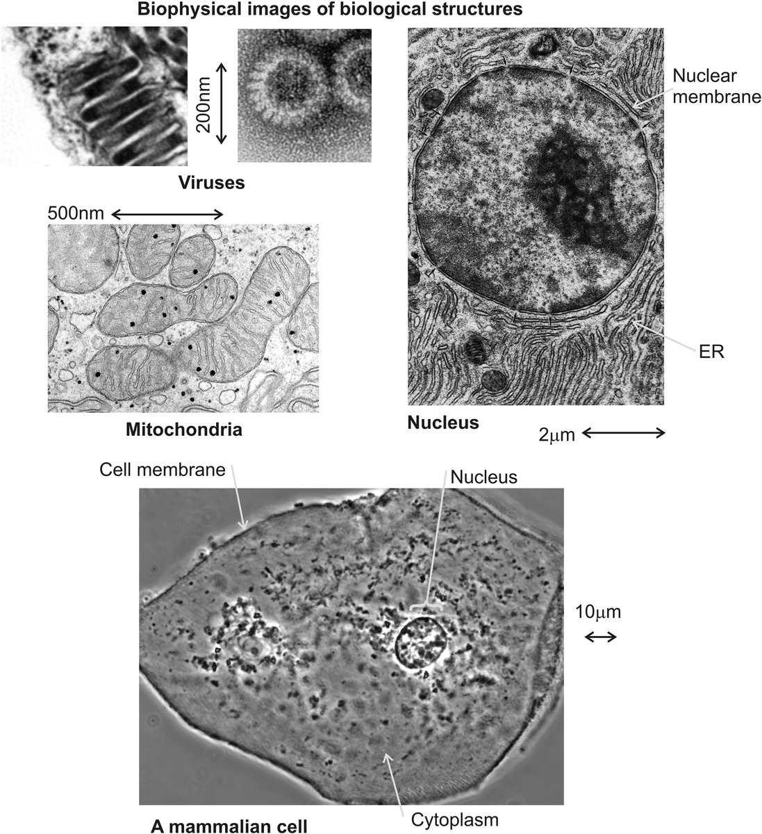
Figure 2.1 The architecture of biological structures. A range of typical cellular structures, in addition to viruses. (a) Rodlike maize mosaic viruses, (b) obtained using negative staining followed by transmission electron microscopy (TEM) (see Chapter 5); (c) mitochondria from guinea pig pancreas cells, (d) TEM of nucleus with endoplasmic reticulum (ER), (e) phase contrast image of a human cheek cell. (a: Adapted from Cell Image Library, University of California at San Diego, CIL:12417 c: Courtesy of G.E. Palade, CIL:37198; d: Courtesy of D. Fawcett, CIL:11045; e: Adapted from CIL:12594.)
2.3 Chemicals that Make Cells Work
Several different types of molecules characterize living matter. The most important of these is undeniably water, but, beyond this, carbon compounds are essential. In this section, we discuss what these chemicals are.
2.3.1 Importance of Carbon
Several different atomic elements have important physical and chemical characteristics of biological molecules, but the most ubiquitous is carbon (C). Carbon atoms, belonging to Group IV of the periodic table, have a normal typical maximum valency of 4 (Figure 2.2a) but have the lowest atomic number of any Group IV element, which imparts not only a relative stability to carbon–carbon covalent bonds (i.e., bonds that involve the formation of dedicated molecular bonding electron orbitals) compared to other elements in that group such as silicon, which contain a greater number of protons in their nuclei with electrons occupying outer molecular orbitals more distant from the nucleus, but also an ability to form relatively long chained molecules, or to catenate (Figure 2.2b). This property confers a unique versatility in being able to form ultimately an enormous range of different molecular structures, which is therefore correlated to potential biological functions, since the structural properties of these carbon-based molecules affect their ability to stably interact, or not, with other carbon-based molecules, which ultimately is the primary basis of all biological complexity and determinism (i.e., whether or not some specific event, or set of events, is triggered in a living cell).
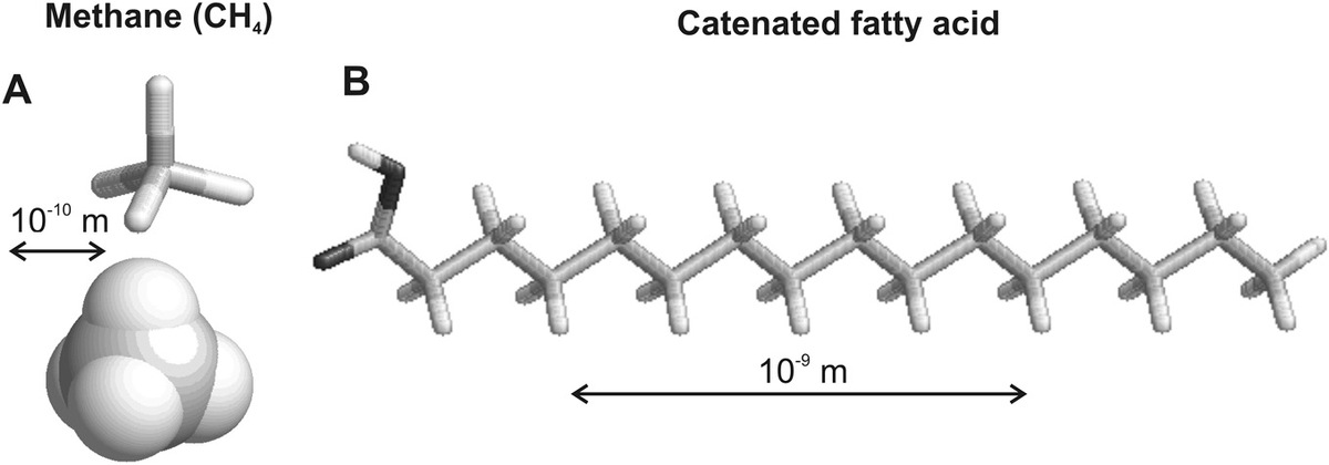
Figure 2.2 Carbon chemistry. (a) Rod and space-filling tetrahedral models for carbon atom bound to four hydrogen atoms in methane. (b) Chain of carbon atoms, here as palmitic acid, an essential fatty acid.
The general field of study of carbon compounds is known as “organic chemistry,” to differentiate it from inorganic chemistry that involves noncarbon compounds, but also confusingly can include the study of the chemistry of pure carbon itself such as found in graphite, graphene, and diamond. Biochemistry is largely a subset or organic chemistry concerned primarily with carbon compounds occurring in biological matter (barring some inorganic exceptions of certain metal ions). An important characteristic of biochemical compounds is that although the catenated carbon chemistry confers stability, the bonds are still sufficiently labile to be modified in the living organism to generate different chemical compounds during the general process of metabolism (defined as the collection of all biochemical transformations in living organisms). This dynamic flexibility of chemistry is just as important as the relative chemical stability of catenated carbon for biology; in other words, this stability occupies an optimum regime for life.
The chemicals of life, which not only permit efficient functioning of living matter during the normal course of an organism’s life but also facilitate its own ultimate replication into future generations of organisms through processes such as cellular growth, replication, and division can be subdivided usefully into types mainly along the lines of their chemical properties.
2.3.2 Lipids and Fatty Acids
By chemically linking a small alcohol-type molecule called “glycerol” with a type of carbon-based acid that contain typically 20 carbon atoms, called “fatty acids,” fats, also known as lipids, are formed, with each glycerol molecule in principle having up to three sites for available fatty acids to bind. In the cell, however, one or sometimes two of these three available binding sites are often occupied by an electrically polar molecule such as choline or similar and/or to charged phosphate groups, to form phospholipids (Figure 2.3a). These impart a key physical feature of being amphiphilic, which means possessing both hydrophobic, or water-repelling properties (through the fatty acid “tail”), and hydrophilic, or water-attracting properties (through the polar “head” groups of the choline and/or charged phosphate).
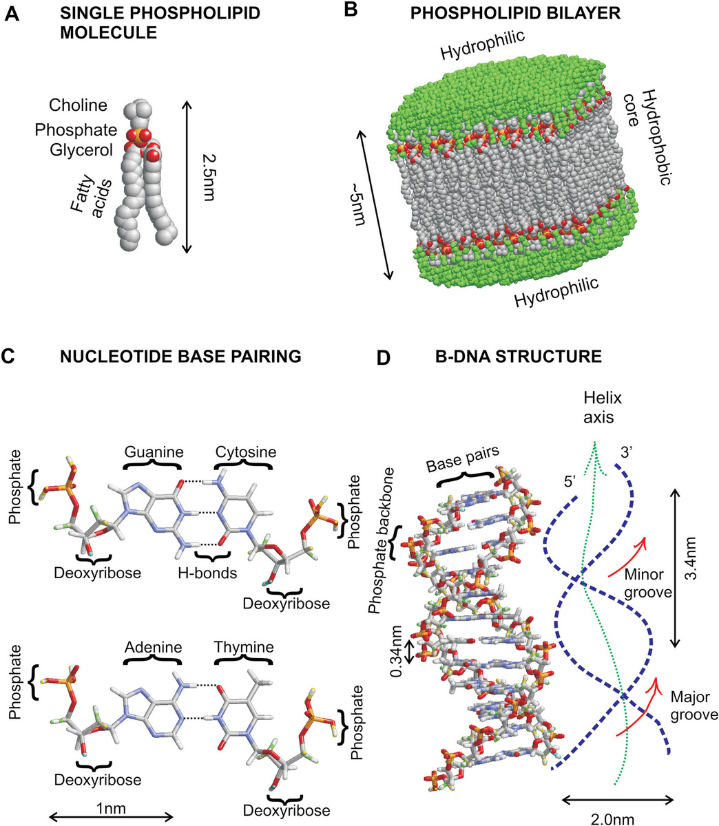
Figure 2.3 Fats and nucleic acids. (a) Single phospholipid molecule. (b) Bilayer of phospholipids in water. (c) Hydrogen-bonded nucleotide base pairs. (d) B-DNA double-helical structure.
This property confers an ability for stable structures to form via self-assembly in which the head groups orientate to form electrostatic links to surrounding electrically polar water molecules, while the corresponding tail groups form a buried hydrophobic core. Such stable structures include at their simplest globular micelles, but more important biological structures can be formed if the phospholipids orient to form a bilayer, that is, where two layers of phospholipids form in effect as a mirror image sandwich in which the tails are at the sandwich center and the polar head groups on the outside above and below (Figure 2.3b). Phospholipid bilayers constitute the primary boundary structure to cells in that they confer an ability to stably compartmentalize biological matter within a liquid water phase, for example, to form spherical vesicles or liposomes (Figure 2.4a) inside cells. Importantly, they form smaller organelles inside the cells such as the cell nucleus, for exporting molecular components generated inside the cell to the outside world, and, most importantly, for forming the primary boundary structure around the outside of all known cells, of the cell membrane, which arguably is a larger length scale version of a liposome but including several additional nonphospholipid components (Figure 2.4b).
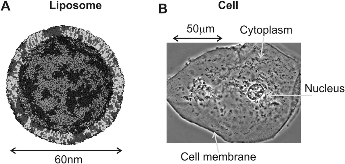
Figure 2.4 Structures formed from lipid bilayers. (a) Liposome, light and dark showing different phases of phospholipids from molecular dynamics simulation (see Chapter 8). (b) The cell membrane and nuclear membranes, from a human cheek cell taken using phase contrast microscopy (Chapter 3).
(a: Courtesy of M. Sansom; b: Courtesy of G. Wright, CIL:12594.)
A phospholipid bilayer constitutes a large free energy barrier to the passage of a single molecule of water. Modeling the bilayer as a dielectric indicates that the electrical permittivity of the hydrophobic core is 5–10 times that of air, indicating that the free energy change, ΔG, per water molecule required to spontaneously translocate across the bilayer is equivalent to ~65 kBT, one to two orders of magnitude above the characteristic thermal energy scale of the surrounding water solvent reservoir. This suggests a likelihood for the process to occur given by the Boltzmann factor of exp(−ΔG/kBT), or ~10−28. Although gases such as oxygen, carbon dioxide, and nitrogen can diffuse in the phospholipid bilayer, it can be thought of as being practically impermeable to water. Water, and molecules solvated in water, requires assistance to cross this barrier, through protein molecules integrated into the membrane.
Cells often have a heterogeneous mixture of different phospholipids in their membrane. Certain combinations of phospholipids can result in a phase transition behavior in which one type of phospholipid appears to pool together in small microdomains surrounded by a sea of another phospholipid type. These microdomains are often dynamic with a temperature-sensitive structure and have been referred to popularly as lipid rafts, with a range of effective diameters from tens to several hundred nanometers, and may have a biological relevance as transient zones of molecular confinement in the cell membrane.
2.3.3 Amino Acids, Peptides, and Proteins
Amino acids are the building blocks of larger important biological polymers called “peptides” or, if more than 50 amino acids are linked together, they are called “polypeptides” or, more commonly, “proteins.” Amino acids consist of a central carbon atom from which is linked an amino (chemical base) group, −NH2, a carboxyl (chemical acid) group, −COOH, a hydrogen atom −H, and one of 23 different side groups, denoted usually as −R in diagrams of their structures (Figure 2.5a), which defines the specific type of amino acid. These 23 constitute the natural or proteinogenic amino acids, though it is possible to engineer artificial side groups to form unnatural amino acids, with a variety of different chemical groups, which have been utilized, for example, in bioengineering (see Chapter 9). Three of the natural amino acids are usually classed as nonstandard, on the basis of either being made only in bacteria and archaea, or appearing only in mitochondria and chloroplasts, or not directly being coded by the DNA, and so many biologists often refer to just 20 natural amino acids, and from these the mean number of atoms per amino acid is 19.
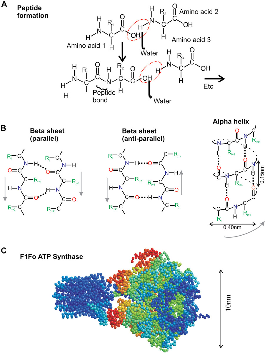
Figure 2.5 Peptide and proteins. (a) Formation of peptide bond between amino acids to form the primary structure. (b) Secondary structure formation via hydrogen bonding to form beta sheets and alpha helices. (c) Example of a complex 3D tertiary structure, here of an enzyme that makes ATP.
It should be noted that theα-carbon atom is described as chiral, indicating that the amino acid is optically active (this is an historical definition referring to the phenomenon that a solution of that substance will result in the rotation of the plane of polarization of incident light). The α-carbon atom is linked in general to four different chemical groups (barring the simplest amino acid glycine for which R is a hydrogen atom), which means that it is possible for the amino acid to exist in two different optical isomers, as mirror images of each other—a left-handed (L) and right-handed (D) isomers—with chemists often referring to optical isomers with the phrase enantiomers. This isomerism is important since the ability for other molecules to interact with any particular amino acid depends on its 3D structure and thus is specific to the optical isomer in question. By far, the majority of natural amino acids exist as l-isomers for reasons not currently resolved.
The natural amino acids can be subdivided into different categories depending upon a variety of physical and chemical properties. For example, a common categorization is basic or acidic depending on the concentration of hydrogen H+ ions when in water-based solution. The chemistry term pH refers to −log10 of the H+ ion concentration, which is a measure of the acidity of a solution such that solutions having low values (0) are strong acids, those having high values (14) are strong bases (i.e., with a low acidity), and neutral solutions have a pH of exactly 7 (the average pH inside the cells of many living organism is around 7.2–7.4, though there can be significant localized deviations from this range).
Other broad categorizations can be done on the basis of overall electrical charge (positive, negative, neutral) at a neutral pH 7, or whether the side groups itself is electrically polar or not, and whether or not the amino acid is hydrophobic. There are also other structural features such as whether or not the side groups contain benzene-type ring structures (termed aromatic amino acids), or the side groups consist of chains of carbon atoms (aliphatic amino acids), or they are cyclic (the amino acid proline).
Of the 23 natural amino acids, all but two of them are encoded in the cell’s DNA genetic code, with the remaining rarer two amino acids called “selenocysteine” and “pyrrolysine” being synthesized by other means. Clinicians and food scientists often make a distinction between essential and nonessential amino acids, such that the former group cannot be synthesized from scratch by a particular organism and so must be ingested in the diet.
Individual amino acids can link through a chemical reaction involving the loss of one molecule of water via their amino and carboxyl group to form a covalent peptide bond. The resulting peptide molecule obviously consists of two individual amino acid subunits, but still has a free −NH2 and −COOH at either end and is therefore able to link at each with other amino acids to form longer and longer peptides. When the number of amino acid subunits in the peptide reaches a semiarbitrary 50, then the resultant polymer is termed a “polypeptide or protein.” Natural proteins have as few as 50 amino acids (e.g., the protein hormone insulin has 53), whereas the largest protein is found in muscle tissue and is called “titin,” possessing 30,000 amino acids depending upon its specific type or isomer. The median number of amino acids per protein molecule, estimated from the known natural proteins, is around 350 for human cells. The specific sequence of amino acids for a given protein is termed as “primary structure.”
Since free rotation is permissible around each individual peptide bond, a variety of potential random coil 3D protein conformations are possible, even for the smallest proteins. However, hydrogen bonding (or H-bonding) often results in the primary structure adopting specific favored generic conformations. Each peptide has two independent bond angles called “phi” and “psi,” and each of these bond angles can be in one of approximately three stable conformations based on empirical data from known peptide sequences and stable phi and psi angle combinations, depicted in clusters of stability on a Ramachandran plot. Hydrogen bonding results from an electron of a relatively electronegative atom, typically either nitrogen −N or oxygen −O, being shared with a nearby hydrogen atom whose single electron is already utilized in a bonding molecular orbital elsewhere. Thus, a bond can be formed whose length is only roughly twice as large as the effective diameter of a hydrogen atom (~0.2 nm), which, although not as strong a covalent bond, is still relatively stable over the 20°C–40°C temperatures of most living organisms.
As Figure 2.5b illustrates, two generic 3D motif conformations can result from the periodic hydrogen bonding between different sections of the same protein primary structure, one in which the primary structure of the two bound sections run in opposite directions, which is called a “β-strand,” and the other in which the primary structure of the two bound sections run in the same direction, which results in a spiral-type conformation called an “α-helix.” Each protein molecule can, in principle, be composed of a number of intermixed random coil regions, α-helices and β-strands, and the latter motif, since it results in a relatively planar conformation, can be manifest as several parallel strands bound together to form a β-sheet, though it is also possible for several β-strands to bond together in a curved conformation to form an enclosed β-barrel that is found in several proteins including, for example, fluorescent proteins, which will be discussed later (see Chapter 3). This collection of random coil regions, α-helices and β-strands, is called the protein’s “secondary structure.”
A further level of bonding can then occur between different regions of a protein’s secondary structure, primarily through longer-range interactions of electronic orbitals between exposed surface features of the protein, known as van der Waals interactions. In addition, there may be other important forces that feature at this level of structural determination. These include hydrophobic/hydrophilic forces, resulting in the more hydrophobic amino acids being typically buried in the core of a protein’s ultimate shape; salt bridges, which are a type of ionic bond that can form between nearby electrostatically polar groups in a protein of opposite charge (in proteins, these often occur between negatively charged, or anionic, amino acids of aspartate or glutamate and positively charged, or cationic, amino acids of lysine and arginine); and the so-called disulfide bonds (–S–S–) that can occur between two nearby cysteine amino acids, resulting in a covalent bond between them via two sulfur (–S) atoms. Cysteines are often found in the core of proteins stabilizing the structure. Living cells often contain reducing agents in aqueous solution, which are chemicals that can reduce (bind hydrogen to or remove oxygen from) chemical groups, including a disulfide bond that would be broken by being reduced back into two cysteine residues (this effect can be replicated in the test tube by adding artificial reducing agents such as dithiothreitol [DTT]). However, the hydrophobic core of proteins is often inaccessible to such chemicals. Additional nonsecondary structure hydrogen bonding effects also occur between sections of the same amino acids, which are separated by more than 10 amino acids.
These molecular forces all result in a 3D fine-tuning of the structure to form complex features that, importantly, define the shape and extent of a protein’s structure that is actually exposed to external water-solvent molecules, that is, its surface. This is an important feature since it is the interface at which physical interactions with other biological molecules can occur. This 3D structure formed is known as the protein tertiary structure (Figure 2.5c). At this level, some biologists will also refer to a protein being fibrous (i.e., a bit like a rod), or globular (i.e., a bit like a sphere), but in general most proteins adopt real 3D conformations that are somewhere between these two extremes.
Different protein tertiary structures often bind together at their surface interfaces to form larger multimolecular complexes as part of their biological role. These either can be separate tertiary structures all formed from the same identical amino acid sequence (i.e., in effect identical subunit copies of each other) or can be formed from different amino acid sequences. There are several examples of both types in all domains of life, illustrating an important feature in regard to biological complexity. It is in general not the case that one simple protein from a single amino acid sequence takes part in a biological process, but more typically that several such polypeptides may interact together to facilitate a specific process in the cell. Good examples of this are the modular architectures of molecular tracks upon which molecular motors will translocate (e.g., the actin subunits forming F-actin filaments over which myosin molecular motors translocate in muscle) and also the protein hemoglobin found in the red blood cells that consists of four polypeptide chains with two different primary structures, resulting in two α-chains and two β-chains. This level of multimolecular binding of tertiary structures is called the “quaternary structure.”
Proteins in general have a net electrical charge under physiological conditions, which is dependent on the pH of the surrounding solution. The pH at which the net charge of the protein is zero is known as its isoelectric point. Similarly, each separate amino acid residue has its own isoelectric point.
Proteins account for 20% of a cell by mass and are critically important. Two broad types of proteins stand out as being far more important biologically than the rest. The first belongs to a class referred to as enzymes. An enzyme is essentially a biological catalyst. Any catalyst functions to lower the effective free energy barrier (or activation barrier) of a chemical reaction and in doing so can dramatically increase the rate at which that reaction proceeds. That is the simple description, but this hides the highly complex detail of how this is actually achieved in practice, which is often through a very complicated series of intermediate reactions, resulting in the case of biological catalysts from the underlying molecular heterogeneity of enzymes, and may also involve quantum tunneling effects (see Chapter 9). Enzymes, like all catalysts, are not consumed per se as a result of their activities and so can function efficiently at very low cellular concentrations. However, without the action of enzymes, most chemical reactions in a living cell would not occur spontaneously to any degree of efficiency over the time scale of a cell’s lifetime. Therefore, enzymes are essential to life. (Note that although by far the majority of biological catalysts are proteins, another class of catalytic RNA called “ribozymes” does exist.) Enzymes in general are named broadly after the biological process they primarily catalyze, with the addition of “ase” on the end of the word.
The second key class of proteins is known as molecular machines. The key physical characteristic of any general machine is that of transforming energy from one form into some type of mechanical work, which logically must come about by changing the force vector (either in size or direction) in some way. Molecular machines in the context of living organisms usually take an input energy source from the controlled breaking of high-energy chemical bonds, which in turn is coupled to an increase in the local thermal energy of surrounding water molecules in the vicinity of that chemical reaction, and it is these thermal energy fluctuations of water molecules that ultimately power the molecular machines.
Many enzymes act in this way and so are also molecular machines; however, at the level of the energy input being most typically due to thermal fluctuations from the water solvent, one might argue that all enzymes are types of molecular machines. Other less common forms of energy input are also exhibited in some molecular machines, for example, the absorption of photons of light can induce mechanical changes in some molecules, such as the protein complex called “rhodopsin,” which is found in the retina of eyes.
There are several online resources available to investigate protein structures. One of these includes the Protein Data Bank (www.pdb.org); this is a data repository for the spatial coordinates of atoms of measured structures of proteins (and also some biomolecule types such as nucleic acids) acquired using a range of structural biology tools (see Chapter 5). There are also various biomolecule structure software visualization and analysis packages available. In addition, there are several bioinformatics tools that can be used to investigate protein structures (see Chapter 8), for example, to probe for the appearance of the same sequence repeated in different sets of proteins or to predict secondary structures from the primary sequences.
2.3.4 Sugars
Sugars are more technically called “carbohydrates” (for historical reasons, since they have a general chemical formula that appears to consist of water molecules combined with carbon atoms), with the simplest natural sugar subunits being called “monosaccharides” (including sugars such as glucose and fructose) that mostly have between three and seven carbon atoms per molecule (though there are some exceptions that can have up to nine carbon atoms) and can in principle exist either as chains or in a conformation in which the ends of the chain link to each other to form a cyclic molecule. In the water environment of living cells, by far the majority of such monosaccharide molecules are in the cyclic form.
Two monosaccharide molecules can link to each other through a chemical reaction, similar to the way in which a peptide bond is formed between amino acids by involving the loss of a molecule of water, but here it is termed as glycosidic bond, to form a disaccharide (Figure 2.6a). This includes sugars such as maltose (two molecules of glucose linked together) and sucrose (also known as table sugar, the type you might put in your tea, formed from linking one molecule of glucose and one of fructose).
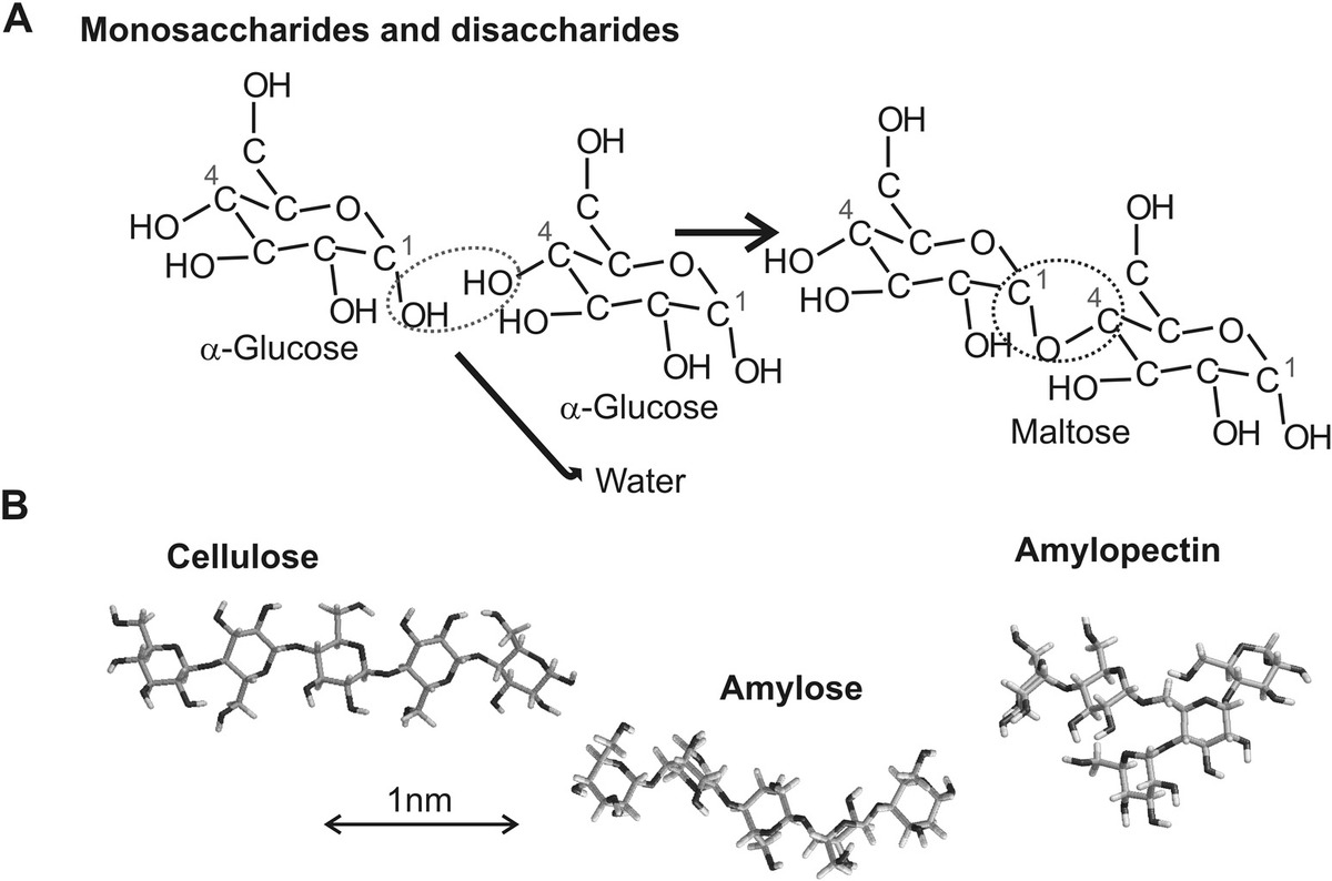
Figure 2.6 Sugars. (a) Formation of larger sugars from monomer units of monosaccharide molecules via loss of water molecule to form a disaccharide molecule. (b) Examples of polysaccharide molecules.
All sugars contain at least one carbon atom which is chiral, and therefore can exist as two optical isomers; however, the majority of natural sugars exist (confusingly, when compared with amino acids) as the –D form. Larger chains (Figure 2.6b) can form from more linkages to multiple monosaccharides to form polymers such as cellulose (a key structural component of plant cell walls), glycogen (an energy storage molecule found mainly in muscle and the liver), and starch.
These three examples of polysaccharides happen all to be comprised of glucose monosaccharide subunits; however, they are all structurally different from each other, again illustrating how subtle differences in small features of individual subunits can be manifest as big differences as emergent properties of larger length scale structures. When glucose molecules bind together, they can do so through one of two possible places in the molecule. These are described as either 1 → 4 or 1 → 6, referring to the numbering of the six carbon atoms in the glucose molecule.
In addition, the chemical groups that link to the glycosidic bond itself are in general different, and so it is again possible to have two possible stereoisomers (a chemistry term simply describing something that has the same chemical formula but different potential spatial arrangements of the constituent atoms), which are described as either α or β; cellulose is a linear chain structure linked through β(1 → 4) glycosidic bonds containing as few as 100 and as high as a few thousand glucose subunits; starch is actually a mixture of two types of polysaccharide called “amylose” linked through mainly α(1 → 4) glycosidic bonds, and amylopectin that contains α(1 → 4) and as well as several α(1 → 6) links resulting in branching of the structure; glycogen molecules are primarily linked through α(1 → 4), but roughly for every 10 glucose subunits, there is an additional link of α(1 → 6), which results in significant branching structure.
2.3.5 Nucleic Acids
Nucleic acids include molecules such as DNA and various forms of RNA. These are large polymers composed of repeating subunits called “nucleotide bases” (Figure 2.3c) characterized by having a nucleoside component, which is a cyclic molecule containing nitrogen as well as carbon in a ringed structure, bound to a five-carbon-atom monosaccharide called either “ribose,” in the case of RNA, or a modified form of ribose lacking a specific oxygen atom called “deoxyribose,” in the case of DNA, in addition to bound phosphate groups. For DNA, the nucleotide subunits consist of either adenine (A) or guanine (G), which are based on a chemical structure known as purines, and cytosine (C) or thymine (T), which are based on a smaller chemical structure known as pyrimidines, whereas for RNA, the thymine is replaced by uracil (U).
The nucleotide subunits can link to each other in two places, defined by the numbered positions of the carbon atoms in the structure, in either the 3′ or the 5′ position (Figure 2.3d), via a nucleosidic bond, again involving the loss of a molecule of water, which still permit further linking of additional nucleotides from both the end 3′ and 5′ positions that were not utilized in internucleotide binding, which can thus be subsequently repeated for adding more subunits. In this way, a chain consisting of a potentially very long sequence of nucleotides can be generated; natural DNA molecules in live cells can have a contour length of several microns.
DNA strands have an ability to stably bind via base pair interactions (also known as Watson–Crick base pairing) to another complementary strand of DNA. Here, the individual nucleotides can form stable multiple hydrogen bonds to nucleotides in the complementary strand due to the tessellating nature of either the C–G (three internucleotide H-bonds) or A–T (two internucleotide H-bonds) structures, generating a double-helical structure such that the H-bonds of the base pairs span the axial core of the double helix, while the negatively charged phosphate groups protrude away from the axis on the outside of the double helix, thus providing additional stability through minimization of electrostatic repulsion.
This base pairing is utilized in DNA replication and in reading out of the genetic code stored in the DNA molecule to make proteins. In DNA replication, errors can occur spontaneously from base pairing mismatch for which noncomplementary nucleotide bases are paired, but there are error-checking machines that can detect a substantial proposal of these errors during replication and correct them. Single-stranded DNA can exist, but in the living cell, this is normally a transient state that is either stabilized by the binding of specific proteins or will rapidly base pair with a strand having a complementary nucleotide sequence.
Other interactions can occur above and below the planes of the nucleotide bases due to the overlap of delocalized electron orbitals from the nucleotide rings, called “stacking interactions,” which may result in heterogeneity in the DNA helical structures that are dependent upon both the nucleotide sequence and the local physical chemistry environment, which may result in different likelihood values for specific DNA structures than the base pairing interactions along might suggest. For the majority of time under normal conditions inside the cell, DNA will adopt a right-handed helical conformation (if the thumb of your right hand was aligned with the helix axis and your relaxed, index finger of that hand would follow the grooves of the helix as they rotate around the axis) called “B-DNA” (Figure 2.3d), whose helical width is 2.0 nm and helical pitch is 3.4 nm consisting of a mean of 10.5 base pair turns. Other stable helical conformations exist including A-DNA, which has a smaller helical pitch and wider width than B-DNA, as well as Z-DNA, which is a stable left-handed double helix. In addition, more complex structures can form through base pairing of multiple strands, including triple-helix structures and Holliday junctions in which four individual strands may be involved.
The importance of the phosphate backbone of DNA, that is, the helical lines of phosphate groups that protrude away from the central DNA helix to the outside, should not be underestimated, however. A close inspection of native DNA phosphate backbones indicate that this repeating negative charge is not only used by certain enzymes to recognize specific parts of DNA to bind to but perhaps more importantly is essential for the structural stability of the double helix. For example, replacing the phosphate groups chemically using noncharged groups results in significant structural instability for any DNA segment longer than 100 nucleotide base pairs. Therefore, although the Watson–Crick base pair model includes no role for the phosphate background in DNA, it is just as essential.
The genetic code is composed of DNA that is packaged into functional units called “genes.” Each gene in essence has a DNA sequence that can be read out to manufacture a specific type of peptide or protein. The total collection of all genes in a given cell in an organism is in general the same across different tissues in the organism (though note that some genes may have altered functions due to local environmental nongenetic factors called “epigenetic modifications”) and referred to as the genome. Genes are marked out by start (promoter) and end points (stop codon) in the DNA sequence, though some DNA sequences that appear to have such start and end points do not actually code for a protein under normal circumstances. Often, there will be a cluster of genes between a promoter and stop codon, which all get read out during the same gene expression burst, and this gene cluster is called an “operon.”
This presence of large amounts of noncoding DNA has accounted for a gradual decrease in the experimental estimates for the number of genes in the human genome, for example, which initially suggested 25,000 genes has now, at the time of writing, been revised to more like 19,000. These genes in the human genome consist of 3 × 10⁹ individual base pairs from each parent. Note, the proteome, which is the collection of a number of different proteins in an organism, for humans is estimated as being in the range (0.25–1) × 106, much higher than the number of genes in the genome due to posttranscriptional modification.
DNA also exhibits higher-order structural features, in that the double helix can stably form coils on itself, or the so-called supercoils, in much the same way as the cord of a telephone handset can coil up. In nonsupercoiled, or relaxed B-DNA, the two strands twist around the helical axis about once every 10.5 base pairs. Adding or subtracting twists imposes strain, for example, a circular segment of DNA as found in bacteria especially might adopt a figure-of-eight conformation instead of being a relaxed circle. The two lobes of the figure-of-eight conformation are either clockwise or counterclockwise rotated with respect to each other depending on whether the DNA is positively (overwound) or negatively (underwound) supercoiled, respectively. For each additional helical twist being accommodated, the lobes will show one more rotation about their axis.
In living cells, DNA is normally negatively supercoiled. However, during DNA replication and transcription (which is when the DNA code is read out to make proteins, discussed later in this chapter), positive supercoils may build up, which, if unresolved, would prevent these essential processes from proceeding. These positive supercoils can be relaxed by special enzymes called “topoisomerases.”
Supercoils have been shown to propagate along up to several thousand nucleotide base pairs of the DNA and can affect whether a gene is switched on or off. Thus, it may be the case that mechanical signals can affect whether or not proteins are manufactured from specific genes at any point in time. DNA is ultimately compacted by a variety of proteins; in eukaryotes these are called “histones,” to generate higher-order structures called “chromosomes.” For example, humans normally have 23 pairs of different chromosomes in each nucleus, with each member of the pair coming from a maternal and paternal source. The paired collection of chromosomes is called the “diploid” set, whereas the set coming from either parent on its own is the haploid set.
Note that bacteria, in addition to some archaea and eukaryotes, can also contain several copies of small enclosed circles of DNA known as plasmids. These are separated from the main chromosomal DNA. They are important biologically since they often carry genes that benefit the survival of the cell, for example, genes that confer resistance against certain antibiotics. Plasmids are also technologically invaluable in molecular cloning techniques (discussed in Chapter 7).
It is also worth noting here that there are nonbiological applications of DNA. For example, in Chapter 9, we will discuss the use of DNA origami. This is an engineering nanotechnology that uses the stiff properties of DNA over short (ca. nanometer distances) (see Section 8.3) combined with the smart design principles offered by Watson–Crick base pairing to generate artificial DNA-based nanostructures that have several potential applications.
RNA consists of several different forms. Unlike DNA, it is not constrained solely as a double-helical structure but can adopt more complex and varied structural forms. Messenger RNA (mRNA) is normally present as a single-stranded polymer chain of typical length of a few thousand nucleotides but potentially may be as high as 100,000. Base pairing can also occur in RNA, rarely involving two complementary strands in the so-called RNA duplex double helices, but more commonly involving base pairing between different regions of the same RNA strand, resulting in complex structures. These are often manifested as a short motif section of an RNA hairpin, also known as a stem loop, consisting of base pair interactions between regions of the same RNA strand, resulting in a short double-stranded stem terminated by a single-stranded RNA loop of typically 4–8 nucleotides. This motif is found in several RNA secondary structures, for example, in transfer RNA (tRNA), there are three such stem loops and a central double-stranded stem that result in a complex characteristic clover leaf 3D conformation. Similarly, another complex and essential 3D structure includes rRNA. Both tRNA and rRNA are used in the process of reading and converting the DNA genetic code into protein molecules.
One of the subunits of rRNA (the light subunit) has catalytic properties and is an example of an RNA-based enzyme or ribozyme. This particular ribozyme is called “peptidyl transferase” that is utilized in linking together amino acids during protein synthesis. Some ribozymes have also been demonstrated to have self-replicating capability, supporting the RNA world hypothesis, which proposes that RNA molecules that could self-replicate were in fact the precursors to life forms known today, which ultimately rely on nucleic acid-based replication.
2.3.6 Water and Ions
The most important chemical to life as we know is, undeniably, water. Water is essential in acting as the universal biological solvent, but, as discussed at the start of this chapter, it is also required for its thermal properties, since the thermal fluctuations of the water molecules surrounding molecular machines fundamentally drive essential molecular conformational changes required as part of their biological role. A variety of electrically charged inorganic ions are also essential for living cells in relative abundance, for purposes of electrical and pH regulation, and also as being utilized as in cellular signaling and for structural stability, including sodium (Na+), potassium (K+), hydrogen carbonate (HCO3−), calcium (Ca2+), magnesium (Mg2+), chloride (Cl−), and water-solvated protons (H+) present as hydronium (or hydroxonium) ions (H3O+).
Other transition metals are also utilized in a variety of protein structures, such as zinc (Zn, e.g., present in a common structural motif involving in protein binding called a “zinc finger motif”) as well as iron (Fe, e.g., located at the center of hemoglobin protein molecules used to bind oxygen in the blood). There are also several essential enzymes that utilize higher atomic number transition metal atoms in their structure, required in comparatively small quantities in the human diet but still vital.
2.3.7 Small Organic Molecules of Miscellaneous Function
Several other comparatively small chemical structures also perform important biological functions. These include a variety of vitamins; they are essential small organic molecules that for humans are often required to be ingested in the diet as they cannot be synthesized by the body; however, some such vitamins can actually be synthesized by bacteria that reside in the guts of mammals. A good example is E. coli bacteria that excrete vitamin K that is absorbed by our guts; the living world has many such examples of two organisms benefiting from a mutual symbiosis, E. coli in this case benefiting from a relatively stable and efficacious external environment that includes a constant supply of nutrients.
There are also hormones; these are molecules used in signaling between different tissues in a complex organism and are often produced by specialized tissues to trigger emergent behavior elsewhere in the body. There are steroids and sterols (which are steroids with alcohol chemical groups), the most important perhaps being cholesterol, which gets a bad press in that its excess in the body lead to a well-reported dangerous narrowing of blood vessels, but which is actually an essential stabilizing component of the eukaryote cell membrane.
There are also the so-called neurotransmitters such as acetylcholine that are used to convey signals between the junctions of nerve cells known as synapses. Nucleoside molecules are also very important in cells, since they contain highly energetic phosphate bonds that release energy upon being chemically split by water (a process known as hydrolysis); the most important of these molecules is adenosine triphosphate that acts as the universal cellular fuel.
2.4 Cell Processes
Cells can regulate their behavior, or phenotype, by ultimately controlling the number of protein molecules of different types that are present inside the cell at any one time. This is important since cells inside an organism may all have the same ultimate set of genes made from the DNA inside each of their cell nuclei but may need to perform very diverse roles in the organism. For example, in the human body there are roughly 200 different types of cells, as classified by biological experts, cells that will have different sizes and shapes and have catered biochemical and mechanical properties to be specialized in specific parts of the body, such as in the nerves, bones, muscles, skin, and blood.
Most of the very smallest cells belong to the archaea domain in a genus subdivision also called Mycoplasma, found commonly in soil, which are roughly 200 nm in diameter, very close to the theoretical minimum size predicted on the basis of estimating the length of DNA genetic code in principle required to generate the very barest essential components necessary for a cell to replicate itself and thus be “alive” and using the polymer physics properties of DNA to predict its typical end-to-end distance. Mycoplasma “ghost” cell membranes (cells minus their native DNA genetic material) were also used in generating the first self-replicating artificial cell (Gibson et al., 2010). The longest cells known are nerve cells, which in some animals can be several meters in length.
The way that the number, or ultimately the concentration, of each type of protein molecule in a cell is controlled is through dynamic fine-tuning of the rate of production of proteins and the rate at which they are removed, or degraded, from the cell. There are mechanisms to controllably degrade proteins in cells, for example, eukaryotes have a mechanism of tagging proteins (with another protein called “ubiquitin”), leading to their being ultimately captured inside subcellular organelles and subsequently degraded by the action of the so-called proteolytic enzymes, with other similar mechanisms existing for prokaryotes but with the absence of dedicated subcellular organelles. However, the most control that is imparted by cells for regulating the equilibrium concentration of cellular proteins is through the direct regulation of the rate at which they are manufactured by the cell from the genes. The fine-tuning of the rate of production of proteins in a cell is done through a process called gene regulation, and to understand how this is achieved, we must explore the concept of the central dogma of molecular biology.
2.4.1 Central Dogma of Molecular Biology
For reasons that arguably are more metaphysical than scientific, the process, which is considered by many expert biologists to be the most important of all biology, which governs how the DNA genetic code is ultimately read out and transformed into different proteins, is referred to as a central dogma as opposed to a law. Either way, the process itself is ubiquitous across all domains of life, and essential, summarized in its simplest form in Figure 2.7. In essence, the following applies:
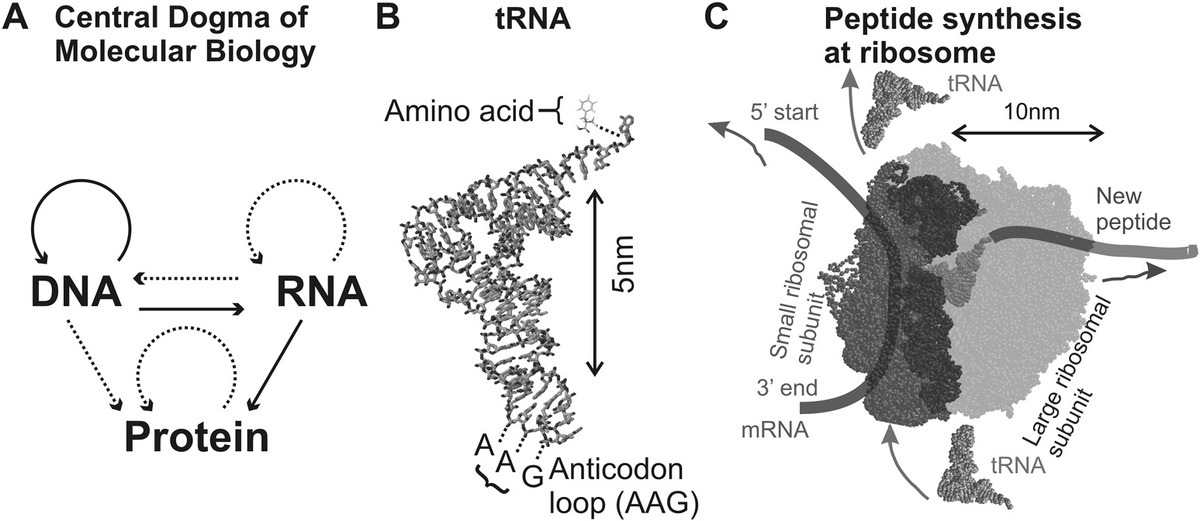
Figure 2.7 Central dogma of molecular biology, (a) Schematic of the flow of information between nucleic acids and proteins. (b) Structure of tRNA. (c) Interaction of tRNA with ribosome during peptide manufacture.
- The genetic code of each cell is encapsulated in its DNA, into a series of genes.
- Genes can be transcribed by molecular machinery to generate molecules of mRNA.
- mRNA molecules can be translated by other molecular machinery involving the binding of molecules of tRNA to the mRNA to generate peptides and proteins.
This is an enormous simplification of what is a very complex process requiring the efficient coordination of multiple different molecular machine components. The principal flow of information from the genes incorporated into DNA molecules to the rest of the organism is through the route DNA → mRNA → protein. The proteins that are then generated can feature in, most importantly, various different enzymes that potentially catalyze thousands of different biochemical reactions in thousands of biological processes in an organism, as well as a vast range of molecular machines that drive a variety of energy-dependent systems inside cells, not to mention an enormous range of essential structural cellular components as well as those involved in the detection of chemical signals both inside and outside the cell.
As Figure 2.7 suggests, there are other mechanisms for information to flow from, and to, nucleic acids, as well as directly from protein to protein. For example, DNA replication, an essential process, which ultimately allows daughter cells from newly divided cells to receive a copy of the parental cell’s genetic code, involves DNA → DNA information flow. Protein → protein information flow can occur through the generation of prions; peptide-based self-replicating structures requiring no direct transfer of information from nucleic acids, which when incorrectly folded, are implicated in various pathologies of the brain including Creutzfeldt–Jakob disease, more commonly referred to by its equivalent disorder in cattle of mad cow’s disease. Note also that there is evidence that correctly folded prions may also have a functional role in information flow. For example, certain damaged nerve cells appear to cleave correctly folded prion molecules whose fragments then act as a signal to neighboring cells called “Schwann cells,” which stimulates them to repair the damaged nerve cell by manufacturing an increased amount of a substance called the “myelin sheath,” which is a fatty-based dielectric that acts as an electrical insulator around nerve cells.
RNA → DNA information flow can occur through an enzyme called “reverse transcriptase,” which is utilized by some types of viruses called “retroviruses” that store their genetic material in the form of RNA but then use reverse transcriptase to convert it to DNA prior to integrating this into the DNA of a host-infected cell (a well-known example is the human immunodeficiency virus [HIV]). RNA → RNA information flow can also occur through a direct replication of RNA from an RNA template using another viral enzyme called “RNA replicase” (studied most extensively in the polio virus).
The key stages of the principal information flow route of DNA → mRNA → protein for the central dogma are as follows:
- A molecular machine enzyme called “RNA polymerase” (RNAP) binds to a specific region of the DNA at the start of a particular gene, called the promoter, whose binding core contains a common nucleotide sequence that is present in all domains of life of 5′-TATAAA-3′ and is also known as the TATA box. A series of proteins called “transcription factors” (TFs) can also compete for binding of the RNAP through specific binding to the particular sequence of a given gene’s promoter region and in doing so can specifically inhibit the binding of the RNAP in the promoter region of that gene. This is thought to be the primary way in which the expression of proteins and peptides from genes, that is, whether or not a gene is switched on, is regulated, in that if a TF is bound to the promoter region, then the gene will not express any protein, and so is switched off, whereas in the absence of any bound TF, the gene is switched on. Expression from a single gene is thus stochastic and occurs in bursts of activity.
- The RNAP is a good example of a multicomponent enzyme. One component is responsible for first unwinding the double helix in the vicinity of the RNAP.
- The RNAP then moves along one of the single strands of DNA specifically in the 3′–5′ direction; this process in itself is highly complex and far from completely understood but is known from a variety of single-molecule experiments performed in a test tube environment (i.e., in vitro techniques) to require a chemical energy input from the hydrolysis of ATP, resulting in molecular conformational changes to the RNAP that fuel its movement along the DNA. The transcription speed along the DNA varies typically from 20 to 90 nucleotides per second (though note that some viruses can adapt the cell’s RNAP to increase its effective speed of transcription by a factor of 20).
- As the RNAP moves along the single strand of DNA, each nucleotide base of the DNA is copied by generating a complementary strand of mRNA.
- Once the RNAP reaches a special stop signal in the DNA code, the copying is stopped and the completed mRNA is released from the RNAP.
- In the case of eukaryotic cells, the mRNA molecule first diffuses out of the nucleus through specialized nanoscale holes in the nuclear membrane called “nucleopores” and can then be modified by enzyme-medicated splicing reactions called posttranscriptional modifications that can result in significant variability from the original mRNA molecule manifested as sequence differences in the proteins or peptides that are ultimately generated. Each eukaryotic gene, in general, consists of coding DNA regions called “exons” interspersed with noncoding regions called “introns,” and splicing of the mRNA involves in effect differential shuffling and relinking of the equivalent exon regions in the mRNA by a complex molecular machine called the “spliceosome.” In prokaryotes, there are no introns and no established mechanisms for posttranscriptional modifications.
- The mRNA molecule, whether modified or not, ultimately then binds to a ribosome in the cytoplasm. Ribosomes are structures roughly 20 nm in average diameter, composed of a mixture of RNA called “rRNA” and proteins. Once bound to a ribosome, the mRNA molecule is translated into a peptide, or protein, sequence, at a typical rate of 8 amino acids per second in eukaryotes, and more likely twice this in prokaryotes.
The mRNA is actually read off in chunks of three consecutive bases, called a “codon.” In principle, this equates to 43, or 64, possible combinations; however, since there are only 20 natural amino acids, there is degeneracy, in that multiple codons may code for the same amino acids (typically between two and six codons exist per amino acid mainly by variation in the third base pair, but two amino acids of methionine in eukaryotes, or formylmethionine in bacteria, and tryptophan are specified by just a single codon). The mRNA sequence for methionine/formylmethionine is denoted AUG, since it consists of adenine, uracil, and guanine, and is a special case since it acts as the start codon in most organisms. Similarly, there are also stop codons (UAA, UAG, and UGA), which consist of other combinations of these three nucleotide bases, also called “nonsense codons or termination codons,” which do not code for an amino acid but terminate mRNA translation. The region between the start and the nearest upstream stop codon is called the “open reading frame,” which generally, but not always, codes for a protein, and in which case is called a “gene.”
Each tRNA molecule acts as an adapter, in that there is a specific tRNA that is attached to each a specific amino acid (Figure 2.7b). Each tRNA molecule then binds via an anticodon binding site to the appropriate codon on the mRNA bound to a ribosome (Figure 2.7c). The general structure of the ribosome consists of a large and small subunit stabilized by base pairing between rRNA nucleotides, which assembles onto the start sequence of each mRNA molecule, sandwiching it together.
The sandwich acts as the site of translation, such that tRNA molecules bind transiently to each active codon and fuse their attached amino acid residues with the nearest upstream amino acid coded by the previous mRNA codon, with the site of active translation on the mRNA shunted forward by moving the mRNA molecule through the ribosome by another codon unit in a process that is energized by the hydrolysis of the molecule GTP (similar to ATP). Multiple ribosomes may bind to the same mRNA molecule to form a polysome (also known as a polyribosome) cluster that can manufacture copies of the same protein from just a single mRNA template each individual ribosome outputting proteins in parallel.
2.4.2 Detection of Signals
Cells can detect the presence of external chemicals with remarkable specificity and efficiency. The typical way this is achieved is through a highly specific receptor that is integrated into the cell membrane composed mainly of protein subunits. The unique 3D spatial conformation adopted by the receptor can allow specific binding of a ligand molecule if it has a conformation that can efficiently fit into the 3D binding site of the receptor; biologists sometimes describe this as a lock-and-key mechanism and is also the way that enzymes are believed to operate on binding to intermediate structures in a biochemical reaction. This correct binding can then trigger subsequent chemical events inside the cell.
The exact mechanism for achieving this is not fully understood but is likely to involve some conformational change to the receptor upon ligand binding. This conversion of the original external chemical signal to inner cellular chemical events is an example of signal transduction. These inner chemical events can then trigger other biological processes and so in effect represents a means of flowing information from the extracellular environment to the inside of the cell. There is scope for similar-shaped molecules outside the cell to compete for binding with the true ligand, and in fact, this is the basis for the action of many pharmaceutical drugs, which are explicitly designed to “block” receptor binding sites in this way.
There is an increasing evidence now for several different cell types possessing an ability to also detect nonchemical signals of mechanical origin. In tightly packed populations of cells, such as in certain tissues and microbial biofilms, the magnitude and direction of mechanical forces are dependent on spatial localization in the matrix of cells. In other words, mechanical signals could potentially be utilized as a cellular metric for determining where it is in relation to other cells. This has relevance to how higher-order multicellular structures emerge from smaller discrete cell components, for example, in microbial biofilms and many different types of animals and plant tissues. As to how such mechanical signals are detected, and ultimately transduced, is not clear. There is evidence of mechanoreceptors whose conformation appears to be dependent on local stresses in the vicinity of its localization in the cell membrane. There is also evidence that mechanical forces on DNA can affect its supercoiling topology in a controlled way.
2.4.3 Trapping “Negative” Entropy
A useful thermal physics view of living matter is that this is characterized by pockets of locally trapped “negative” entropy. The theoretical physicist Erwin Schrödinger wrote a useful treatment on this (Schrödinger, 1944) discussing how life feeds off negative entropy. By this, he was really referring to the concept of minimizing free energy to form a stable state, as opposed to some mysterious quantity of negative entropy per se. Life in essence results in pockets of locally ordered matter. This appears to be decoupled from the spirit of the second law of thermodynamics, though note that we cannot consider biological systems to be thermally closed, and instead when we consider the entropy of the whole universe, this will never decrease due to any biological process. But life can be thought of as being local reductions of entropy.
How is this achieved? What does “life” actually do to create local order? Ultimately, living organisms chemically combine carbon with other chemicals to form the various molecular forms of carbon-based living matter alluded to previously, all of which have greater order than their respective reactants. But where does this carbon come from? Organisms can eat other organisms of course and assimilate their biochemical contents, but somewhere at the very bottom of the food chain, the carbon has to come from a nonbiological source. This involves extracting carbon dioxide from the atmosphere by chemically combining it with water, fueled by energy from the sun, in a process called “photosynthesis,” which occurs in plants and some microbial organisms.
The first key stage in photosynthesis involves an enzyme called “ribulose-1,5-bisphosphate carboxylase oxygenase” (RuBisCO), which is the most abundant known protein on Earth. It catalyzes the reaction of carbon dioxide into a precursor of sugars in a process called the “Calvin cycle,” fueled through ATP hydrolysis. RuBisCO in prokaryotes is often found in specialized cellular organelles of carboxysomes. The initial absorption of light occurs either in the cell membrane directly (in photosynthetic cyanobacteria) or invaginated membrane thylakoids of chloroplasts (in plant eukaryotes) in light-harvesting complexes, which are multiprotein machines that operate as antennae to absorb visible light photons in combination with pigments (e.g., carotenoids and chlorophylls). This results in an effective spatial funneling of the incident photons through transfer of their energy to surrounding molecules via a nonradiative electronic molecular orbital resonance effect that generates high-energy electrons from the photosynthetic reaction center.
Quantum tunneling of these excited electrons (see Chapter 9) occurs in a series of electron transfer reactions with a drop in electron energy coupled at each stage to a series of chemical reactions, which results in the of pumping protons across a membrane in which consequent electrochemical energy is used to fuel the reaction of carbon dioxide with water, to oxygen as a by-product as well as produce small sugar molecules, which lock up the energy of the originally excited electrons into high-energy chemical bonds.
On the basis of simple thermodynamics, for any process to occur spontaneously requires a negative change in free energy, which is a (thermal) nonequilibrium condition. This is true for all processes, including those biological. Living matter in effect delays the dispersion of their free energy toward more available microstates (which moves toward a condition of thermal equilibrium at which the change in free energy is precisely zero) by placing limits on the number of available microstates toward which the free energy can be dispersed. This is achieved by providing some form of continuous energy input into the system.
Ultimately, this energy input comes principally from the sun, though in some archaea, this can be extracted from heat energy from thermal vents deep in the ocean. Another way to view this is that energy inputted into the local thermal system of a living organism is utilized to perform mechanical work in some form to force the system away from its natural tendency of a state of maximum disorder as predicted from the second law, which is done by fueling a variety of subcellular, cellular, and multicellular processes to regulate the organism’s stable internal environment, a process that biologists describe as homeostasis (from the Greek, meaning literally “standing still”).
Either way, this energy is trapped in some chemical form, typically in relatively simple sugar molecules. However, releasing all of the energy trapped in a single molecule of glucose in one go (equivalent to >500 kBT) is excessive in comparison to the free energy changes encountered during most biological processes. Instead, cells first convert the chemical potential energy of each sugar molecule into smaller bite-sized chunks by ultimately manufacturing several molecules of ATP. The hydrolysis of a single molecule of ATP, which occurs normally under catalytic control in the presence of enzymes called “kinases,” will release energy locally equivalent to ~18 kBT, which is then converted into increased thermal energy of surrounding water solvent molecules whose bombardment on biological structures ultimately fuels mechanical changes to biological structures.
This input of free energy into biological systems can be thought of as a delaying tactic, which ultimately only slows down the inevitable process of the system reaching a state of thermal equilibrium, equivalent to a state of maximum entropy, and of death to the biological organism. (Note that many biological processes do exist in a state of chemical equilibrium, meaning that the rate of forward and reverse reactions are equal, as well as several cellular structures existing in a state of mechanical equilibrium, meaning that the sum of the kinetic and potential energy for that structure is a constant.)
But how are ATP molecules actually manufactured? Most sugars can be relatively easily converted in the cell into glucose, which is then broken down into several chemical steps releasing energy that is ultimately coupled to the manufacture of ATP. Minor cellular processes that achieve this include glycolysis as well as fermentation (in plant cells and some prokaryotes), but the principle ATP manufacturing route, generating over 80% of cellular ATP, is via the tricarboxylic acid (TCA) cycle (biologists also refer to this variously as the citric acid, Krebs, or the Szent–Györgyi–Krebs cycle), which is a complex series of chemical reactions in which an intermediate breakdown product of glucose (and also ultimately of fats and proteins) called “acetyl-CoA” is combined with the chemical acetate and then converted in a cyclic series of steps into different organic acids (all characterized as having three –COOH groups, hence the preferred name of the process).
Three of these steps are coupled to a process, which involves the transfer of an electron (in the form of atomic hydrogen H as a bound H+ proton and an electron) to the nucleoside nicotinamide adenine dinucleotide (NAD+), or which ultimately forms the hydrogenated compound NADH, with one of the steps using a similar electron-carrier protein or flavin adenine dinucleotide (FAD+), which is hydrogenated to make the compound FADH (Figure 2.8). The TCA cycle is composed of reversible reactions, but is driven in the direction shown in Figure 2.8 by a relatively high concentration of acetyl-CoA maintained by reactions that breakdown glucose.
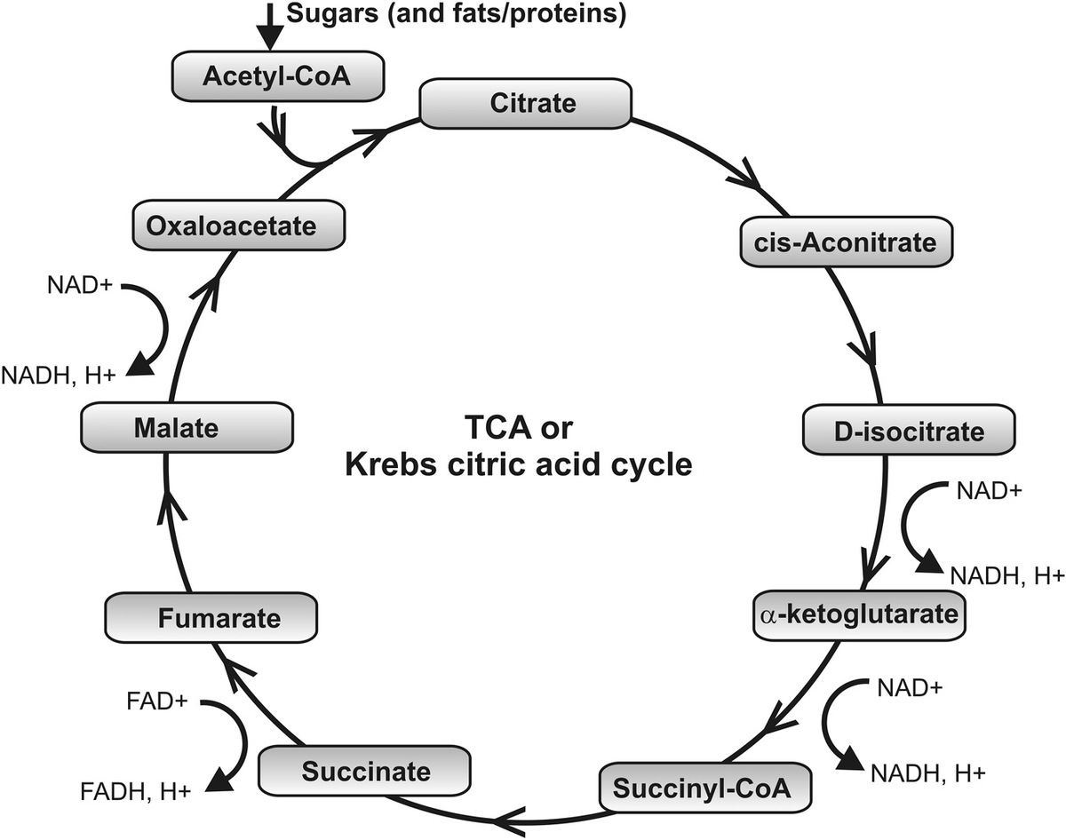
Figure 2.8 Schematic of the tricarboxylic acid or Krebs citric acid cycle.
Prokaryotes and eukaryotes differ in how they ultimately perform the biochemical processes of manufacturing ATP, known generally as oxidative phosphorylation (OXPHOS), but all use proteins integrated into a phospholipid membrane, either of the cell membrane (prokaryotes) or in the inner membrane of mitochondria (eukaryotes). The electron-carrier proteins in effect contain one or more electrons with a high electrostatic potential energy. They then enter the electron transport chain (ETC) and transfer the high-energy electrons to/from a series of different electron-carrier proteins via quantum tunneling (biologists also refer to these electron-carrier proteins as dehydrogenases, since they are enzymes that catalyze the removal of hydrogen). Lower-energy electrons, at the end of the series of ETCs, are ultimately transferred to molecular oxygen in most organisms, which then react with protons to produce water; some bacteria are anaerobic and so do not utilize oxygen, and in these instances an terminal electron acceptor of either sulfur or nitrogen is typically used.
Chemists treat electron gain and electron loss as reduction and oxidation reactions, respectively, and so such a series of sequential electron transfer reactions are also called electrochemical “redox reactions.” Each full redox reaction is the sum of two separate half reactions involving reduction and oxidation, each of which has an associated reduction potential (E0), which is the measure of the equivalent electrode voltage potential if that specific chemical half reaction was electrically coupled to a standard hydrogen electrode (the term standard means that all components are at concentrations of 1 M, but confusingly the biochemical standard state electrode potential is the same as the standard state electrode potential apart from the pH being 7; the pH is defined as −log10[H+ concentration] and thus indicates a concentration of H+ of 10−7 M for the biochemical standard state).
The reduction half reaction for the electron acceptor NAD+ is
(2.1)An example of a reduction half reaction at one point in the TCA cycle (see Figure 2.8) involves an electron acceptor called of “oxaloacetate−,” which is reduced to malate−:
(2.2)These two reversible half reactions can be combined by taking one away from the other, so malate− then acts as an electron donor and in the process is oxidized back to oxaloacetate−, which is exactly what occurs at one point in the TCA cycle (two other similar steps occur coupled to the reduction of NAD+, and another coupled to FAD+ reduction, Figure 2.8). The concentrations of oxaloacetate and malate are kept relatively low in the cell at 50 nM and 0.2 mM, respectively, and these low concentrations compared to the high concentration of acetyl-CoA result in a large excess of NAD+.
A general reduction half reaction can be written as a chemical state O being reduced to a chemical state R:
(2.3) O + nH+ + ne- ⇌ Rwhere the free energy change per mole associated with this process can be calculated from the electrical and chemical potential components:
(2.4)where F is Faraday’s constant, 9.6 × 10⁴ C mol−1, equivalent to the magnitude of the electron charge q multiplied by Avogadro’s number NA, n electrons in total being transferred in the process. This also allows the molar equilibrium constant K to be calculated:
(2.5)where R is the molar gas constant, equal to kBNA, with absolute temperature T. Equation 2.4 can be rewritten by dividing through by −nF:
(2.6)Equation 2.6 is called the “Nernst equation.”
The free energy of oxidation of NADH and FADH is coupled to molecular machines, which pump protons across either the mitochondrial inner membrane (eukaryotes) or cytoplasmic membrane (prokaryotes) from the inside to the outside, to generate a proton motive force (pmf), Vpmf, of typical value −200 mV relative to the inside. The free energy required to pump a single proton against this pmf can be calculated from Equation 2.4 equating Vpmf to E. This proton motive force is then coupled to the rotation of the FoF1–ATP synthase in the membrane to generate ATP. For the TCA cycle, each molecule of glucose is ultimately broken down into a theoretical maximum of 38 molecules of ATP based on standard relative chemical stoichiometry values of the electron-carrier proteins and how many electrons can be transferred at each step, though in practice the maximum number is less in a living cell and more likely to be 30–32 ATP molecules per glucose molecule.
The pmf is an example of a chemiosmotic proton gradient (for a historical insight, see Mitchell, 1961). It constitutes a capacitance electrostatic potential energy. This potential energy can be siphoned off by allowing the controlled translocation of protons down the gradient through highly specific proton channels in the membrane. In a mechanism that is still not fully understood, these translocating protons can push around a paddle-wheel-type structure in a molecular machine called the “FoF1ATP synthase.” The FoF1ATP synthase is a ubiquitous molecular machine in cells composed of several different protein subunits, found inside bacteria, chloroplasts in plants, and most importantly to us humans in mitochondria. The machine itself consists of two coupled rotary motors (see Okuno et al., 2011). It consists of an inner water-soluble F1 motor exposed to the cellular cytoplasm with a rotor shaft protein called γ surrounded by six stator units composed of alternating α and β proteins (Figure 2.5c). There is also an outer hydrophobic Fo motor linked to the rotor shaft. Under more normal conditions, the Fo motor couples the chemiosmotic energy stored in the proton gradient across the cell membrane lipid bilayer to the rotation of the F1 motor that results in ATP being synthesized from ADP and inorganic phosphate (but note that under conditions of oxygen starvation the motors can hydrolyze ATP and rotate in the opposite direction, causing the protons to be pumped up the proton gradient).
2.4.4 Natural Selection, Neo-Darwinism, and Evolution
Neo-Darwinism, which evokes classical natural selection concepts of Darwinism in the context of modern genetics theory, has been described by some life scientists as the central paradigm of biology. The essence of the paradigm is that living organisms experience a variety of selective pressures, and that the organisms best adapted to overcome these pressures will survive to propagate their genetic code to subsequent generations. By a “selective pressure,” biologists mean some sort of local environmental parameter that affects the stochastic chances of an organism surviving, for example, the abundance or scarcity of food, temperature, pressure, the presence of oxygen and water, and the presence of toxic chemicals. In any population of organisms, there is a distribution of many different biological characteristics, which impart different abilities to thrive in the milieu of these various selective pressures, meaning that some will survive for longer than others and thus have a greater chance of propagating their genetic code to subsequent generations either through asexual cell division processes or through sexual reproduction.
This in essence is the nuts and bolts of natural selection theory, but the devil is very much more in the detail! Neo-Darwinism accounts for the distribution in biological characteristics of organisms through genetics, namely, in the underlying variation of the DNA nucleotide sequence of genes. Although the cellular machinery that causes the genetic code in DNA to be replicated includes error-checking mechanisms, there is still a small probability of, for example, a base pairing mismatch error (see Question 2.7), somewhere between 1 in 105 (for certain viruses) and 109 (for many bacteria and eukaryotic cells) per replicated nucleotide pair depending on the cell type and organism. If these errors occur within a gene, then they can be manifested as a mutation in the phenotype due to a change resulting from the physical, chemical, or structural properties of the resulting peptide or protein that is expressed from that particular gene.
Such a change could affect one or more biological processes in the cell, which utilize this particular protein, resulting in an ultimate distribution of related biological properties, depending on the particular nature of the mutated protein. If this mutated DNA nucleotide sequence is propagated into another cellular generation, then this biological variation will also be propagated, and if this cell happens to be a so-called germ cell of a multicellular organism, then this mutation may subsequently be propagated into offspring through sexual reproduction. Hence, selective pressures can bias the distribution of the genetic makeup in a population of cells and organisms of subsequent generations resulting, over many, many generations, in the evolution of that species of organism.
However, there is increasing evidence for some traits, which can be propagated to subsequent cellular generations not through alteration of the DNA sequence of the genetic code itself but manifested as functional changes to the genome. For example, modification of histone proteins that help to package DNA in eukaryotes can result in changes to the expression of the associated gene in the region of the DNA packaged by these histones. Similarly, the addition of methyl chemical groups to the DNA itself are known to affect gene expression, but without changing the underlying nucleotide sequence. The study of such mechanisms is called “epigenetics.” An important factor with many such epigenetic changes is that they can be influenced by external environmental factors.
This concept, on the surface, appears to be an intriguing reversion back to redundant theories exemplified by the so-called Lamarckism, which essentially suggested erroneously that, for example, if a giraffe stretched its neck to reach leaves in a very tall tree, then the offspring from that giraffe in subsequent generations would have slightly longer necks. Although epigenetics does not make such claims, it does open the door to the idea that what an organism experiences in its environment may affect the level of expression of genes in subsequent generations of cells, which can affect the behavior of those cells in sometimes very dramatic ways.
This is most prominently seen in cellular differentiation. The term “differentiation” used by biologists means “changing into something different” and is not to be confused with the term used in calculus. This is the process by which nongerm cells (i.e., cells not directly involved in sexual reproduction, also known as somatic cells) turn into different cell types; these cells all have the same DNA sequence, but there are significant differences in the timing and levels of gene expressions between different cell types, now known to be largely due to epigenetics modifications. This process is first initiated from the so-called stem cells, which are cells that have not yet differentiated into different cell types. The reason why stem cells have such current interest in biomedical applications is that if environmental external physical and chemical triggers can be designed to cause stem cells to controllably and predictably change into specific cell types, then these can be used to replace cells in damaged areas of the body to repair specific physiological functions in humans, for example.
The exact mechanisms of natural selection, and ultimately species evolution, are not clear. Although at one level, natural selection appears to occur at the level of the whole organism, on closer inspection, a similar argument could be made at both larger and smaller length scales. For example, at larger length scales, there is natural selection at the level of populations of organisms, as exhibited in the selfless behavior of certain insects in appearing to sacrifice their own individual lives to improve the survival of the colony as a whole. At a smaller length scale, there are good arguments to individual cells in the same tissue competing with each other for nutrients and oxygen, and at a smaller length scale, still an argument for completion occurring at the level of single genes (for a good background to the debate, see Sterelny, 2007).
An interesting general mechanism is one involving the so-called emergent structures, a phenomenon familiar to physicists. Although the rules of small length and time scale interaction, for example, at the level of gene expression and the interactions between proteins, can be reduced to relatively simple forces, these interactions can lead to higher-order structures of enormous complexity called emergent structures, which often have properties that are difficult to predict from the fundamental simple sets of rules of individual interacting units. There is good evidence that although evolution is driven at the level of DNA molecules, natural selection occurs at the level of higher-order emergent structures, for example, cells, organisms, colonies, and biofilms. This is different from the notion that higher-order structures are simply “vehicles” for their genes, though some biologists refer to these emergent structures as extended phenotypes of the gene. This area of evolutionary biology is still hotly contested with some protagonists in the field formulating arguments, which, to the lay observer, extend beyond the purely scientific, but what is difficult to deny is that natural selection exists, and that it can occur over multiple length scales in the same organism at the same time.
The danger for the physicist new to biology is that in this particular area of the life sciences, there is a lot of “detail.” Details are important of course, but these sometimes will not help you get to the pulsing heart of the complex process, that is, adaptation from generation to generation in a species in response the external environment. Consider, instead, an argument more aligned with thermal physics:
This, of course, does not “explain” evolution, but it is not a bad basis from which the physicist has to start at least. Evolutionary change is clearly far from simple, however.
One very common feature, which many recent research studies have suggested, which spans multiple length scales from single molecules up through to cells, tissues, whole organisms, and even ecologies of whole organisms, seems to be that of a phenomenon known as bet hedging. Here, there is often greater variability in a population than one might normally expect on the grounds of simple efficiency considerations—for example, slightly different forms of a structure of a given molecule, when energetically it may appear to be more efficient to just manufacture one type. This variability is in one sense a form of “noise”; however, in many cases, it confers robustness to environmental change, for example, by having multiple different molecular forms that respond with different binding kinetics to a particular ligand under different conditions, and in doing so that organism may stand a greater chance of survival even though there was a greater upfront “cost” of energy to create that variability. Unsurprisingly, this increase in noise is often seen in systems of particularly harsh/competitive environmental conditions.
Note that although natural selection when combined with variation in biological properties between a competing population, at whatever disputed length scale, can account for aspects of incremental differences between subsequent generations of cell cycles and organism life spans, and ultimately evolutionary change in a population, this should not be confused with teleological/teleonomic arguments. In essence, these arguments focus on the function of a particular biological feature. One key difference in language between biology and physics is the use of the term “function”—in physics we use it to mean a mapping between different sets of parameters, whereas in biology the meaning is more synonymous with purpose or role. It is not so much that new features evolve to perform a specific role, though some biologists may describe it as such, rather that selective pressure results in better adaptation to a specific set of environmental conditions.
Also, natural selection per se does not explain how “life” began in the first place. It is possible to construct speculative arguments on the basis, for example, of RNA replicators being the “primordial seed” of life, which forms the basis of the RNA world hypothesis. RNA is a single-stranded nucleic acid unlike the double-stranded DNA and so can adopt more complex 3D structures, as seen, for example, in the clover leaf shape of tRNA molecules and in the large complex RNAP, both used in transcribing the genetic code. Also, RNA can form a version of the genetic code, seen in RNA viruses and in mRNA molecules that are the translated versions of coding DNA. Thus, RNA potentially is an autocatalyst for its own replication, with a by-product resulting in the generation of peptides, which in turn might ultimately evolve over many generations into complex enzymes, which can catalyze the formation of other types of biological molecules. There is a further question though of how cell membranes came into being since these are essential components of the basic cellular unit of life. However, there is emerging evidence that micelles, small, primordial lipid bilayer vesicles, may also be autocatalytic, that is, the formation of a micelle makes it more likely for micelles to form further. But a full discussion of this theory and others of creation myths of even greater speculation are beyond the scope of this book but are discussed by Dawkins and elsewhere.
2.4.5 “Omics” Revolution
Modern genetics technology has permitted the efficient sequencing of the full genome of several organisms. This has enabled the investigation of the structure, function of, and interactions between whole genomes. This study is genomics. The equivalent investigation between the functional interactions of all the proteins in an organism is called “proteomics.” Many modern biophysical techniques are devoted to genomics and proteomics investigations, which are discussed in the subsequent chapters of this book. There are now also several other omics investigations. Epigenomics is devoted to investigating the epigenome, which is the collection of epigenetics factors in a given organism. Metabolomics studies the set of metabolites within a given organism. Other such fields are lipidomics (the characterization of all lipids in an organism), similarly transcriptomics (the study of the collected set of all TFs in an organism), connectomics (study of the neural connections), and several others. An interesting new omics discipline is mechanomics (Wang et al., 2014); this embodies the investigation of all mechanical properties in an organism (especially so at the level of cellular mechanical signal transduction), which crosses into gene regulation effects, more conventionally thought to be in the regime of transcriptomics, since there is now emerging evidence of mechanical changes to the cell being propagated at the level of the local structure of DNA and affecting whether genes are switched on or off. Arguably, the most general of the omics fields of study is that called simply “interactomics”; this investigates the interactome, which is the collection of all interactions within the organism and so can span multiple length and time scales and the properties of multiple physical parameters and, one could argue, embodies the collection of all other omics fields.
2.5 Physical Quantities in Biology
Many of the physical quantities in biological systems have characteristic origins and scales. Also, part of the difference in language between physical scientists and biologists involves the scientific units in common use for these physical quantities.
2.5.1 Force
The forces relevant to biology extend from the high end of tissue supporting the weight of large organisms; adult blue whales weigh ~200 tons, and so if the whale is diving at terminal velocity, the frictional force on the surface will match its weight, equivalent to 2 × 10⁶ N. For plants, again the forces at the base of a giant sequoia tree are in excess of 1 × 10⁷ N. For humans, the typical body weight is several hundred newtons, so this total force can clearly be exerted by muscles in legs. However, such macrolength scale forces are obviously distributed throughout the cells of a tissue. For example, in muscle, the tissue may be composed of 10–20 muscle fibers running in parallel, each of which in turn might be composed of ~10 myofibrils, which are the equivalent cellular level units in muscle. With the additional presence of connective tissue in between the fibers, the actual cellular forces are on the order of sub-newtons. This level of force can be compared with that required to break a covalent chemical bond such as a carbon–carbon bond of ~10−9 N, or a weaker noncovalent bond such as those of an antibody binding of ~10−10 N.
At the lower end of the scale are forces exerted by individual molecular machines, typically around the level of a few multiples of 10−12 N. This unit is the piconewton (pN), which is often used by biologists. The weakest biologically relevant forces in biology are due to random thermal fluctuations of surrounding water-solvent molecules, which is an example of the Langevin force (or fluctuation force), depending upon the length and time scale of observation. For example, a nucleus of diameter ~10−6 m observed for a single second will experience a net Langevin force of ~10−14 N. Note that in biology, gravitational forces of biological molecules are normally irrelevant (e.g., ~10−17 N).
One of the key attractive forces, which are essential to all organisms, is that of covalent bonding, which allows strong chemical bonds to form between atoms, of carbon in particular. Covalent bonds involve the sharing of pairs of electrons from individual atomic orbitals to form stable molecular orbitals. The strength of these bonds is often quantified by the energy required to break them (as the bond force integrated over the distance of the bond). The bond energy involving carbon atoms typically varies in a range of 50–150 kBT energy units.
Cells and biomolecules are also affected by several weaker noncovalent forces, which can be both attractive and repulsive. An ideal way to characterize a vector force F is through the grad function of the respective potential energy landscape of that force, U:
(2.7)Electrostatic forces in the water-solvated cellular environment involve layers of polar water molecules and ions, in addition to an electrical double layer (EDL) (the Gouy–Chapman layer) composed of ions adsorbed onto molecular surfaces with a second more diffuse weakly bound to counter charges of the first layer. The governing equation for the electrostatic potential energy is governed by Coulomb’s law, which in its simplest form describes the electric potential Ve due to a single point of charge q at a distance r:
(2.8)where
- ε0 is the electrical permittivity in a vacuum
- εm is the relative electrical permittivity in the given medium
Therefore, for example, for two charges of equal magnitude q but opposite sign, separated by a distance d, each will experience an attractive electrostatic force Fe toward the other parallel to the line that joins the two charges of
(2.9)For dealing with multiple electrical charges in a real biological system, a method called “Ewald summation” is employed, which treats the total electrical potential energy as the sum of short-range and long-range components. The usual way to solve this often complex equation is to use the particle mesh Ewald method (PME method), which treats the short-range and long-range components separately in real space and Fourier space (see Chapter 8).
Van der Waals forces (dispersion-steric repulsion), as discussed, are short-range steric repulsive potential energy with 1/r12 (distance r) dependence fundamentally due to the Pauli exclusion principle in quantum mechanics. The exclusion principle disallows the overlap of electron orbitals. When we combine this short-range repulsive component with a longer-range attractive component from interactions with nonbonding electrons inducing electrical dipoles, a 1/r6 dependence, we get the so-called “Lennard–Jones potential,” which is also referred to as the L-J, 6-12, and 12-6 potential) UL-J:
(2.10)Here, A and B are the constants of the particular biological system.
Hydrogen (or H–) bonding, already referred to, is a short-range force operating over ~0.2–0.3 nm. These are absolutely essential to forming the higher-order structures of many different biological molecules. The typical energy required to break an H-bond is ~5kBT.
Hydrophobic forces are largely entropic based resulting from the tendency of nonpolar molecules to pool together to exclude polar water molecules. There is no simple law to describe hydrophobic forces, but they are the strongest at 10–20 nm distances, and so are generally perceived as long range. Hydrophobic bonds are very important in stabilizing the structural core of globular protein molecules.
Finally, there are Helfrich forces. These result from the thermal fluctuations of cell membranes due to random collisions of solvent water molecules. They are a source entropic force, manifest as short-range repulsion.
2.5.2 Length, Area, and Volume
At the high end of the biological length scale, for single organisms at least, is a few tens of meters (e.g., the length of the largest animal is the blue whale at ~30 m, the largest plant is the giant sequoia tree at almost 90 m in height). Colonies of multiple organisms, and whole ecosystems, can clearly be much larger still. At the low end of the scale are single biological molecules, which are typically characterized by a few nanometers (unit nm or 10−9 m; i.e., 1 m/1000 million) barring exceptions such as filamentous biopolymers, like DNA, which can be much longer. Crystallographers also use a unit called the “Angstrom” (Å), equal to 10−10 m, since this is the length scale of the hydrogen atom diameter, and so typical covalent and hydrogen bond lengths will be a few Angstroms.
Surface area features investigated in biology often involve cell membranes, and since the length scale of cell diameter is typically a few microns (μm), the μm2 area unit is not uncommon. For volume, biochemistry in general refers to liter units (L) of 10−3 m3, but typical quantities for biochemical assays often involve volumes in the range 1–1000 μL (microliters), though more bulk assays potentially use several milliliters (mL).
2.5.3 Energy and Temperature
Molecular scale (pN) forces integrated over with nanometer spatial displacements result in an energy scale of a few piconewton nanometers. The piconewton nanometer unit (pN nm) equals 10−21 J.
Organisms have a high temperature, from a physics perspective, since quantum energy transitions are small relative to classical levels, and so the equipartition theorem, that each independent quadratic term, or degree of freedom, in the energy equation for a molecule in an ensemble at absolute temperature T has an average energy kBT/2. A water molecule has three translational, three rotational, and three intrinsic vibrational energy modes (note each vibrational mode has two degrees of freedom of potential and kinetic energy) plus up to three additional extrinsic vibrational modes since each atom can, in principle, independently form a hydrogen bond with another nearby water molecule, indicating a mean energy of ~9 kBT per molecule.
Following collision with a biological molecule, some of this kinetic energy is transferred, resulting in kBT scale energy fluctuations; kBT itself is often used by biologists as a standard unit of energy, equivalent to 4.1 pN nm at room temperature. This is roughly the same energy scale as molecular machines undergoing typical displacement transitions of a few nanometers through forces of a few piconewtons. This is because molecular machines have evolved to siphon-off energy from the thermal fluctuations of surrounding water to fuel their activity. The hydrolysis of one molecule of ATP in effect releases 18 kBT of chemical potential energy from high-energy phosphate bonds to generate thermal energy.
Note that some senior biologists still refer to an energy unit of the calorie (cal). This is defined as the energy needed to raise the temperature of 1 g of water through 1°C at a pressure of one atmosphere. Intuitively, from the discussion earlier, this amount of energy, at room temperature, is equivalent to 4.1 J. Many bond energies, particularly in older, but still useful, biochemistry textbooks are often quoted in units of kcal.
The temperature units used by most biologists are degrees Celsius (°C), that is, 273.15 K higher than absolute temperature. Warm-blooded animals have stable body temperatures around 35°C–40°C due to complex thermoregulation mechanisms, but some may enter hibernation states of more like 20°C–30°C. Many cold-blooded animals thrive at a room temperature of 20°C, and some plants can accommodate close to the full temperature range of liquid water. Microbes have a broad range of optimal temperatures; many lie in the range of 20°C–40°C, often optimized for living in the presence of, or symbiotically with, other multicellular organisms. However, some, including the so-called extremophiles, many from the archaea domain of organisms, thrive at glacial water temperatures in the range 0°C–5°C, and at the high end some can thrive at temperatures of 80°C–110°C either in underwater thermal vents or in atmospheric volcanic extrusions. The full temperature range when considered across all organisms broadly reflects the essential requirement of liquid water for all known forms of life. Many proteins begin to denature above 50°C, which means that their tertiary and quaternary structures are disrupted through the breaking of van der Waals interactions, with the result of the irreversible change of their 3D structure and thus, in general, destruction of their biological function.
There are some well-known protein exceptions that occur in types of extremophile cells that experience exceptionally high temperatures, known as thermophiles. One such is a thermophilic bacterium called Thermus aquaticus that can survive in hot water pools, for example, in the vicinity of lava flow, to mean temperatures of 80°C. An enzyme called “Taq polymerase,” which is naturally used by these bacteria in processing of DNA replication, is now routinely used in polymerase chain reactions (PCR) to amplify a small sample of DNA, utilized in biomedical screening and forensic sciences, as well as being routinely used in abundance for biological research (see Chapter 7). A key step in PCR involves cycles of heating up replicated (i.e., amplified) DNA to 90°C to denature the two helical strands from each DNA molecule, which each then acts as a template for the subsequent round of amplification, and Taq polymerase facilitates this replication at a rate >100 nucleotide base pairs per second. The advantage of the Taq polymerase is that, unlike DNA polymerases from non-thermophilic organisms, it can withstand such high heating without significant impairment, and in fact even at near boiling water temperatures of 98°C, it has a stability half-life of 10 min.
2.5.4 Time
Time scales in biology are broad. Ultimately, the fastest events are quantum mechanical concerning electronic molecular orbitals, for example, a covalent bond vibrates with a time scale of 10−15 s, but arguably the most rapid events, which make detectable differences to biomolecular components, are collisions from surrounding water molecules, whose typical separation time scale is 10−9 s. Electron transfer processes between molecules are slower at 10−6 s.
Molecular conformational changes occur over more like 10−3 s. Molecular components also turnover typically over a time scale from a few seconds to several minutes. The lifetime of molecules in cells varies considerably with cell type, but several minutes to hours is not atypical. Cellular lifetimes can vary from minutes through years, as therefore do organism lifetimes, though certain microbial spores can survive several hundred million years. Potentially, the range of time scale for biological activity, at a conservative estimate, is ~20 orders of magnitude. In exceptional cases, some biological molecules go into quiescent states and remain dormant for potentially up to several hundred million years. In principle, the complete time scale could be argued to extend from 10−15 s up to the duration over which life is thought to have existed on Earth—4 billion years, or 1018 s.
2.5.5 Concentration and Mass
Molecules can number anything from just 1 to 10 per cell, up to over 104, depending on the type of molecule and cell. The highest concentration, obviously involving the largest number of molecules in the smallest cells, is found in some proteins in bacteria that contain several tens of thousands of copies of a particular protein (many bacteria have a typically small diameter of 1 μm). Biologists often refer to concentration as molarity (M), which is the number of moles (mol) of a substance in 1 L of water solvent, such that 1 mol equals Avogadro’s number of particles (6.022 × 10²³, the number of atoms of the C-12 isotope present in 12 g of pure carbon-12). Typical cellular molarity values for biological molecules are 10−9 M or nanomolar (nM). Some biologists also cite molality, which is the moles of dissolved substance divided by the solvent mass used in kg (units mol kg−1). Dissolved salts in cells have higher concentrations, for example, the concentration of sodium chloride in a cell is about 200 mM (pronounced millimolar) that is also equal in this case to a “200 millimolal” molality.
Mass, for biochemical assays, is often referred to in milligram units (mg). The molecular mass, also called the “molecular weight” (Mw), is the mass of the substance in grams, which contains Avogadro’s number of molecules, but is cited in units of the Dalton (Da) or more commonly for proteins the kilodalton (kDa). For example, the mean molecular weight taken from all the natural amino acids is 137 Da. The largest single protein is an isomer of titin that has a molecular weight of 3.8 MDa. The “molecular weight” of a single ribosome is 4.2 MDa, though note that a ribosome is really not a single molecule but is a complex composed of several subunits. Mass concentration is also used by biologists, typical units of being how many milligrams of that substance is dissolved in an milliliters of water, or milligrams per milliliter (mg mL−1; often pronounced “miggs per mill”).
An alternative unit, which relates to mass but also to length scale, is the svedberg (S, sometimes referred to as Sv). This is used for relatively large molecular complexes and refers to the time it takes to sediment the molecule during centrifugation (see Chapter 6), and so is dependent on its mass and frictional drag. A common example of this includes ribosomes, and their component subunit; the prokaryote ribosome is 70 S. The svedberg is an example of a sedimentation coefficient (see Chapter 6), which is the ratio of a particle’s acceleration to its speed and which therefore has the dimensions of time; 1 S is equivalent to exactly 100 femtoseconds (i.e., 100 fs or 10−13 s). Svedberg units are not directly additive, since they depend both on the mass of the components and to their fractional drag with the surrounding fluid environment that scales with the exposed surface area, which obviously depends on how separate components are bound together in a complex. When two or more particles bind together, there is inevitably a loss of surface area. This can be seen again in the case of the ribosome; the 70 S prokaryotic ribosome has a sedimentation coefficient of 70 S, but is composed of a large subunit of 50 S and a small subunit of 30 S (which in turn includes the 16 S rRNA subunit).
The concentration of protons [H+] is one of the most important measures in biology, though in practice, as discussed, a proton in a liquid aqueous environment, such as inside a cell, is generally coupled through hydrogen bonding to a water molecule as the hydronium/hydroxonium ion H3O+. As discussed, the normal biological representation of proton concentration is as −log10[H+], referred to as the pH, with neutral pH = 7, acids <7, and bases (or alkalis) >7 assuming [H+] is measured in M units.
2.5.6 Mobility
The wide speed range of different biological features obviously reflects the broad time scale of the process in life. At the molecular end of the biology length scale, a key speed measure is that of the translocation of molecular machines, which is typically in the range of a few microns per second, μm s−1. In the cellular regime, there are motile cells, such as self-propelling bacteria that swim an order of magnitude faster. And then at the whole organism scale, there are speeds of more like meters per second, m s−1.
To characterize the net flow of matter due to largely random motions, we talk about diffusion, which has a dimensionality not the same as that of speed, which is [L]/[T], but rather of [L]2/[T], and so conceptually more equivalent to rate at which an “area” is explored in a given time. For purely random-walk behavior of particles, we say that they are exhibiting Brownian diffusion (or normal diffusion). The effective Brownian diffusion coefficient of a biomolecule, D, assuming free and unrestricted diffusion, relates to the variation of effective frictional drag coefficient, γ, through the Stokes–Einstein relation of
(2.11)For the simple case of a sphere of radius r diffusing in a fluid of viscosity η (sometimes referred to more fully as the “dynamic” viscosity, to distinguish it from the “kinematic” viscosity, which is the dynamic viscosity divided by the fluid density), γ is given by 6πηr. This is often a good approximation for a globular-like protein diffusing in the cytoplasm, however different biomolecules in different environments need to be approximated with different shape factors (for example, integrated membrane proteins in a lipid bilayer will typically rotate rapidly over a microsecond timescale or faster perpendicular to the plane of the membrane, and so the effective shape when averaged over a timescale of millisecond or more, which is appropriate for typical light microscopy sampling, is closer to a cylinder perpendicular to the membrane).
In the watery part of the cell, such as the cytoplasm, values of D of a few μ2m s−1 are typical, whereas for a molecule integrated into phospholipid bilayer membranes (30% of all proteins come into this category), the local viscosity is higher by a factor of 100–1000, with resultant values of D smaller by this factor. The theoretical mean squared displacement 〈R2〉, after a time t of a freely diffusing particle in n-dimensional space (e.g., in the cytoplasm n = 3, in the cell membrane n = 2, for a molecular motor diffusing on track, for example, a kinesin molecule on a stiff microtubule filament track, n = 1) is given by
(2.12)But note, in reality, blurring within experimental time sample windows as well as detection precision error leads to a correction for experimental measurements, which involve single particle tracking, and also note that in general there can be several other more complex modes of diffusion inside living cells due to the structural heterogeneity of the intracellular environment.
2.6 Summary Points
- Carbon chemistry permits catenated compounds that form the chemicals of life.
- Biology operates at multiple length and time scales that may overlap and feedback in complex ways.
- The cell is a fundamental unit of life, but in general it needs to be understood in the context of several other cells, either of the same or different types.
- Even simple cells have highly localized architecture, which facilitates specialist biological functions.
- The most important class biomolecules are biological catalysts called “enzymes,” without which most chemical reactions in biology would not happen with any degree of efficiency.
- The shape of molecules is formed from several different forces, which leads to differences in their functions.
- The key process in life is the central dogma of molecular biology, which states that proteins are coded from a genetic code written in the base pair sequence of DNA.
Questions
- 2.1 In a reversible isomerization reaction between two isomers of the same molecule, explain what proportion of the two isomers might be expected to exist at chemical equilibrium, and why. In an autocatalytic reaction, one of the reacting molecules itself acts as a catalyst to the reaction. Explain what might happen with a small excess of one isomer to the relative amounts of each isomer as a function of time. How is this relevant to the d/l isomers amino acids and sugars? Discuss how might evolution affect the relative distribution of two isomers? (For a relevant, interesting read, see Pross, 2014.)
- 2.2 Staphylococcus aureus is a spherical bacterium of 1 μm diameter, which possesses just one circular chromosome. A common form of this bacterium was estimated as having 1.2% of its cellular mass taken up by DNA.
- What is the mass of the cell’s chromosome?
- The bases adenine, cytosine, guanine, and thymine have molecular weights of 0.27, 0.24, 0.28, and 0.26 kDa, respectively, excluding any phosphate groups. The molecular weight of a phosphate group is 0.1 kDa. Estimate the contour length of the S. aureus genome, explaining any assumptions.
- 2.3 The primary structure of a human protein compared to that of budding yeast, S. cerevisiae, which appears to carry out the same specific biological function, was found to have 63% identical sections of amino acids based on short sequence sections of at least five consecutive amino acids in length. However, the respective DNA sequences were found to be only 42% identical. What can account for the difference?
- 2.4 The cell doubling time, a measure of the time for the number of cells in a growing population to double, for E. coli cells, which is a rich nutrient environment, is 20 min. What rate of translation of mRNA into amino acids per second can account for such a doubling time? How does this compare to measured rates of mRNA translation? Comment on the result.
- 2.5 What is the relation between force and its potential energy landscape? Why is it more sensible to consider the potential energy landscape of a particular force first and then deduce the force from this, as opposed to considering just a formulation for the force directly?
- 2.6 What are the van der Waals interactions, and how do these relate to the Lennard–Jones potential? Rewrite the Lennard–Jones potential in terms of the equilibrium distance rm in which the net force is zero and the depth of potential parameter is in Vm, which is the potential energy at a distance rm.
- 2.7 A DNA molecule was found to have a roughly equal mix of adenine, cytosine, guanine, and thymine bases.
- Estimate the probability for generating a mismatched base pair in the DNA double helix, stating any assumptions you make. (Hint: use the Boltzmann factor.) When measured in a test tube, the actual mismatch error was found to be 1 in 105. Comment on the result.
- In a living cell, there is typically one error per genome per generation (i.e., per cell division). What error does this equate to for a human cell? How, and why, does this compare with the value obtained earlier?
- 2.8 Calculate, with reasoning, the free energy difference in units of kBT required to translocate a single sodium ion Na+ across a typical cell membrane. Show, by considering the sodium ion to be a unitary charge q spread over a spherical shell of radius r, that the activation energy barrier required to spontaneously translocate across the lipid bilayer of electrical relative permittivity εr is given by q/8π rεrε0. (Note, this is known as the “electrical self energy”). There is an initial concentration of 150 mM of sodium chloride both inside and outside a roughly spherical cell of diameter 10 μm, with a sodium ion diameter of 0.2 nm. The cell is immersed in a specific kinase inhibitor that prevents ATP hydrolysis, which is normally required to energize the pumping of sodium ions across the cell membrane through sodium-specific ions channels (see Chapter 4), and the cell is then suddenly immersed into pure water. Calculate the number of Na+ ions that the cell loses due solely to spontaneous translocation across the phospholipid bilayer. State any assumptions you make. (The electrical permittivity in a vacuum is 8.9 × 10⁻¹² C2 m−2 N−2, the relative electrical permittivity of a phospholipid bilayer is 5, and the charge on a single electron is −1.6 × 10⁻¹⁹ C.)
- 2.9 The complete oxidation of a single molecule of glucose to carbon dioxide and water in principle involves a total free energy change equivalent of −2870 kJ mol−1 (the minus sign indicates that energy is released, as opposed to absorbed), whereas that for ATP hydrolysis to ADP and inorganic phosphate (the opposite of ATP synthesis) is equivalent to 18 kBT per molecule.
- If the TCA cycle synthesizes a total of 38 ATP molecules from every molecule of glucose, what is the energetic efficiency?
- If ATP synthesis occurs inside a mitochondrion whose volume is comparable to a bacterial cell and the concentration of glucose it utilizes is 5 mM, calculate the theoretical rise in temperature if all glucose were instantly oxidized in a single step. Comment on the result in light of the actual cellular mechanisms for extracting chemical energy from glucose.
- 2.10 At one point in the TCA inside a mitochondrion in a eukaryotic cell cycle, NAD+ is reduced to NADH oxaloacetate−, and the free energy of NADH is coupled to the pumping of a proton across the inner membrane against the proton motive force.
- How much free energy in units of kBT per molecule is required to pump a single proton across the inner membrane?
- Write down this full electrochemical for the reduction of NAD+ by oxaloacetate− and calculate the standard free energy change for this process in units of kBT per molecule. Stating any assumptions, calculate how many protons NADH pump across the inner membrane in a single TCA cycle.
- Inside a mitochondrion, the pH is regulated at 7.5. If all nicotinamide is present either as NAD+ or NADH, calculate the relative % abundance of NAD+ or NADH in the mitochondrion. Comment on the result.
- 2.11 The definition of a cell as outlined in this chapter is as being the minimal structural and functional unit of life that can self-replicate and can exist “independently.” But in practice, a cell is not isolated, for example, there are pores in the membrane that convey molecules in/out of the cell. Does this alter our notion of independence? Are there more robust alternative definitions of a cell?
- 2.12 There are ~1015 cells in a typical human body, but only ~1014 of them are human. What are the others? Does this alter our view of the definition of a “human organism”?
- 2.13 If you go to the Protein Data Bank (www.pdb.org), you can download “pdb” coordinates for many, many molecular structures, the following PDB IDs being good examples: 1QO1 and 1AOI. You can install a variety of free software tools (e.g., RasMol, but there are several others available) and open/display these pdb files.
- Where appropriate, use the software to display separate strands of the DNA double helix red and blue, with nonpolar amino acids residues yellow and polar amino acid residues magenta.
- Using the software, find out what is the maximum separation of any two atoms in either structure.
- 2.14
- What are the attractive and repulsive forces relevant to single biomolecule interactions, and how do they differ in terms of the relative distance dependence and magnitude?
- What forces are most relevant to protein folding of a protein, and why?
- 2.15 The average and standard deviation of heights measured from a population of adult women of the same age and ethnic background were 1.64 and 0.07 m, respectively. Comment on how this compares to the expected variation between the sets of genes from the same population.
- 2.16 A 10 mL of culture containing a virus that infects bacteria was prepared from a culture of growing E. coli bacteria at the peak of viral infection activity, and 1 mL of the culture was divided into 10 volumes of 100 μL each. Nine of these were grown with nine separate fresh uninfected bacterial cultures; all of these subsequently developed viral infections. The 10th volume was then added to fresh culture medium to make up to the same 100 μL volume as the original virus culture and mixed. This diluted virus culture was divided into 10 equal volumes as before, and the previous procedure repeated up to a total of 12 such dilutions. In the first nine dilutions, all nine fresh bacterial cultures subsequently developed virus infections. In the 10th dilution, only six of the nine fresh bacterial cultures developed viral infections; in the 11th dilution, only two of the nine bacterial cultures developed viral infections; and in the 12th dilution, none of the nine bacterial cultures developed viral infection.
- Estimate the molarity of the original virus culture.
- If this culture consisted of virus particles tightly packed, such that the outer coat of each virus was in contact with that of its nearest neighbors, estimate the diameter of the virus. (Hint: a virus culture is likely to cause a subsequent infection of a bacteria culture if there is at least one virus in the culture.)
- 2.17 A key feature of biology is that components of living matter appear to have specific functions. However, the laws of physics are traditionally viewed as being objective and devoid of “purpose.” Discuss this apparent contradiction.
- 2.18 Liquid–liquid phase-separated biomolecular condensates appear to have a preferred length scale in cells, whereas “abiotic” classical nucleation theory for the phase transition process predicts that a transition would, given sufficient time, go to completion until all the relevant molecules are demixed. What reasons can you think of that could account for this difference?
- 2.19 Video-rate fluorescence microscopy with a sampling time of 40 ms per image frame could track a membrane-integrated protein reasonably well, however, images of a similar sized fluorescently labeled protein in the cytoplasm using similar microscopy looked blurry and couldn’t be tracked. Why is this?
References
Key Reference
- Alberts, B. et al. (2008). Molecular Biology of the Cell, 5th ed. Garland Science, New York.
More Niche References
- Banani, S.F. et al. (2017). Biomolecular condensates: organizers of cellular biochemistry. Nat Rev. Mol. Cell Biol. 18:285–298.
- Dawkins, R. (1978). The Selfish Gene, 30th Anniversary ed. (May 16, 2006). Oxford University Press, Oxford, U.K.
- Gibson, D.G. et al. (2010). Creation of a bacterial cell controlled by a chemically synthesized genome. Science 329:52–56.
- Mitchell, P. (1961). Coupling of phosphorylation to electron and hydrogen transfer by a chemi-osmotic type of mechanism. Nature 191:144–148.
- Okuno, D., Iino, R., and Noji, H. (2011). Rotation and structure of FoF1-ATP synthase. J. Biochem. 149:655–664.
- Pross, A. (2014). What Is Life?: How Chemistry Becomes Biology. Oxford University Press, Oxford, U.K.
- Schrödinger, E. (1944). What Is Life—The Physical Aspect of the Living Cell. Cambridge University Press, Cambridge, U.K. Available at http://whatislife.stanford.edu/LoCo_files/What-is-Life.pdf. Accessed on 1967.
- Sterelny, K. (2007). Dawkins vs. Gould: Survival of the Fittest (Revolutions in Science), 2nd revised ed. Icon Books Ltd., Cambridge, U.K.
- Wang, J. et al. (2014) Mechanomics: An emerging field between biology and biomechanics. Protein Cell 5:518–531.